Confusion Matrix

The confusion matrix is a basic instrument in machine learning used to evaluate the performance of classification models. Unlike other performance measures, it provides insight into the nature of the classification errors by illustrating the match and mismatch between the predicted values and the corresponding true values. It is usually a 2x2 table and can be extended to multi-class classification problems.

In the following I will briefly address the structure of the confusion matrix and then illustrate through an example how to generate it using python libraries sklearn and seaborn. However, before I proceed with the confusion matrix, I would like to say a few words about hypothesis testing, since it seems that null hypothesis is often mixed up with the alternative hypothesis.

Null vs Alternative Hypothesis

A hypothesis is an assumption about a population parameter, for example: The average adult drinks 1.7 cups of coffee per day. This statement may or may not be true. The purpose of hypothesis testing is to make a statistical conclusion about accepting or not accepting such statements.

In statistical hypothesis testing, two hypotheses always compete against each other, namely the null and the alternative hypothesis. The alternative hypothesis (\(H_a\)) asserts something and the null hypothesis (\(H_0\)) exactly the opposite. In research, usually the alternative hypothesis expresses the research hypothesis and the null hypothesis asserts that the research hypothesis is not true.

All hypothesis tests have both \(H_0\) and \(H_a\).

Source: ThoughtCo

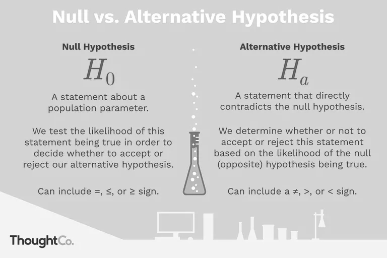
\(H_0\) (read as “H zero” or “H naught”) represents the status quo, it implies a statement that expects no effect or no relationship between two variables. So, in the context of a clinical trial, the null hypothesis would be that a new drug has no effect on a disease. The null hypothesis is believed to be true unless there is overwhelming evidence to the contrary. It is always the hypothesis that is tested.

\(H_a\) usually expresses the research hypothesis and \(H_0\) asserts that the research hypothesis is not true. It is the \(H_0\) that the researcher tries to disprove, whereas an alternative hypothesis is what the researcher wants to prove. A null hypothesis can only be rejected or fail to be rejected; it can not be accepted because of a lack of evidence to reject it. When rejecting the null hypothesis, the alternative hypothesis must be considered.

The courtroom provides a good analogy for a hypothesis test: When a defendant stands trial for a crime, he or she is innocent until proven guilty. \(H_0\) is that the defendant is innocent. \(H_a\) is that the defendant is guilty. The jury presumes \(H_0\) to be true unless the evidence (data) suggests otherwise.

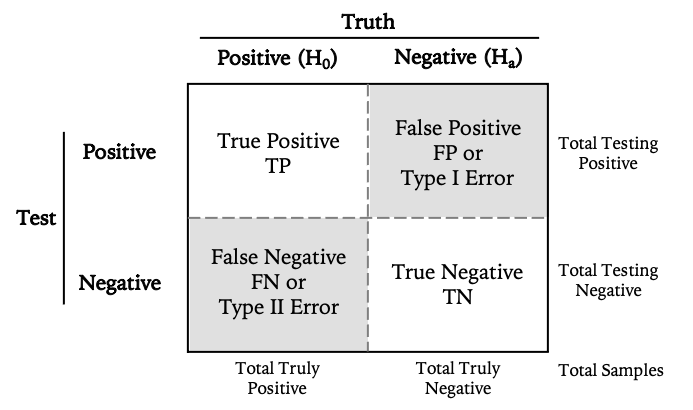
Structure of the confusion matrix

For a binary classification problem, we have a 2x2 matrix, where the rows represent the predicted class and the columns the actual class. The first column represents the Null Hypothesis and the second column is the alternative Hypothesis or the negation to Null Hypothesis.

Let’s now take Covid-19 test as example. The null hypothesis of any diagnostic test of a virus and the associated disease, is that a negative test is presumed, namely:

\(H_0 :=\) No confirmation of the virus.

So the confusion matrix should look like follows:

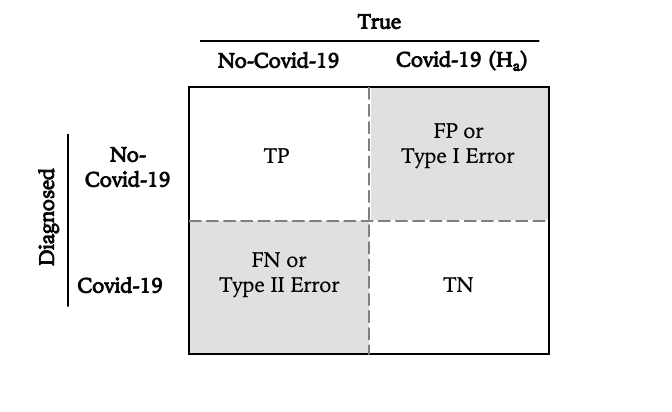
where:

True Positives (TP): the number of Non-Covid-19 patients correctly identified as without Covid-19 by the test
False Positives (FP): the number of patients incorrectly predicted as without Covid-19 —also known as type I Error
False Negatives (FN): the number of patients without Covid-19 incorrectly predicted as with Covid-19 —also known as type II Error
True Negatives (TN): the number of patients with Covid-19 correctly diagnosed.

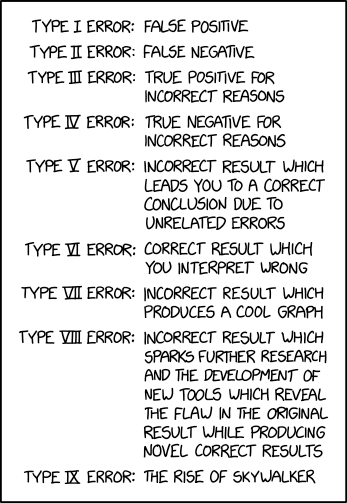
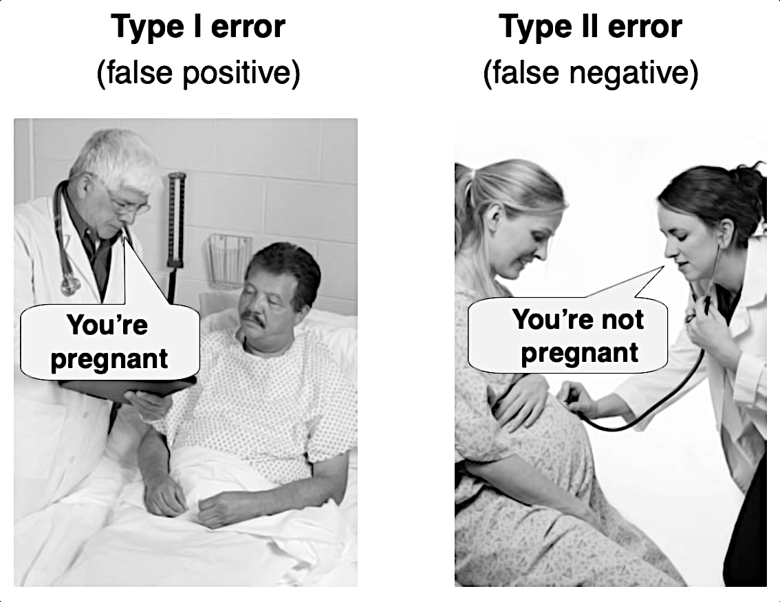
In other words, Covid-19 test can make two types of errors:

Type I: The test result says the patient has Covid-19, but he or she actually doesn’t.
Type II: The test result says the patient doesn’t have Covid-19 virus, but he or she actually does.

A confusion matrix is also nothing but a convenient way of displaying this information. That’s all there is to it… But why do we need to differentiate between different kinds of classification errors?

Not All Errors Are the Same

Source: xkcd

Understanding the difference between type I and type II errors is extremely important, because there’s a risk of making each type of error in every analysis and depending on the situation, the consequences of some errors are worse than others and the amount of risk regarding each is in your control.

Type I error - seeing things that in fact aren’t there - is the rejection of a true null hypothesis and tend to occur more easily than one might think. Indeed, the human brain is hardwired to recognize patterns and draw conclusions even when faced with total randomness. In terms of the courtroom analogy, this error corresponds to convicting an innocent defendant.

A Type II error, or not seeing things that are there, is the failure to reject a false null hypothesis. In terms of the courtroom analogy, a type II error corresponds to acquitting a criminal.

Source: The Essential Guide to Effect Sizes (p. 50)

Imagine you’re a doctor specialized in testing patients for Covid-19. Which error would have more consequences than the other? An FP diagnosis or an FN?

Clearly, the type II error here is the much bigger problem. Both for the person, and for the society. Your objective is to get Covid-19 patients as early as possible. Even if few are not, we can do the test again, but you don’t want to miss early Covid-19 patients. So False Negative (When a patient is having the disease and our model saying he is fine) is something we want to minimize as low as possible. How about classification errors in the criminal justice? Or breath alcohol test? What error has more consequences than the other?

Confusion Matrix in Python

We start first by importing all needed libraries and methods:

import numpy as np
import pandas as pd
import matplotlib.pyplot as plt
from sklearn.metrics import confusion_matrix, classification_report
import seaborn as sns

import random
import warnings

Then we configure our jupyter notebook:

# Set up Notebook
%matplotlib inline
warnings.filterwarnings('ignore')
sns.set_style('white')

# set random seed to ensure reproducibility
random.seed(23)

Now let’s generate dependent and independent data consisting of 0 and 1. Since our null hypothesis states that the patient is covid-19 uninfected we define 0 as negative test results while 1 as positive test results:

# Let's generate some data consisting of random distributed {0, 1}
# where: 
# 0 means: negative test result, and
# 1 means: positive or sick

n_tot = 50 # total number of patients
n_sick = 22 # actual number of sick patients
n_healthy = n_tot - n_sick # actual number of healthy patients
negatives = 5 # Total number of errors (Type I + Type II)
labels = [0, 1] # as in the data

# actual data
y_true = [0]*n_healthy + [1]*n_sick
random.shuffle(y_true) # shuffle data

# prediction or diagnostic:
errors = [0]*(n_tot - negatives) + [1]* negatives
random.shuffle(errors)
y_pred = [abs(x - y) for x, y in zip(y_true, errors)]

Now that we generated y_true and y_pred, we can obtain the confusion matrix by calling the method confusion_matrix() from the sklearn library. So easy is that:

cm = confusion_matrix(y_true, y_pred, labels)
cm

array([[25,  3],
       [ 2, 20]])

Since a picture is worth a thousand words, let’s plot the obtained confusion matrix. To do so, we use the following convenience function:

# Convenience function to plot confusion matrix
def plot_cm(cm, labels):
    """
    This method produces a colored heatmap that displays the relationship
    between predicted and actual class.
    """

    # For simplicity we create a new DataFrame for the confusion matrix
    pd_pts = pd.DataFrame(cm, index=labels, columns=labels )
    
    # Display heatmap and add decorations
    hm = sns.heatmap(pd_pts, annot=True, fmt="d", cbar=False)
    hm.axes.set_title("Confusion Matrix\n", fontsize=20)
    hm.axes.set_xlabel('True Label', fontsize=18)
    hm.axes.set_ylabel('Predicted Label', fontsize=18)

    return None

We now just need to pass the confusion matrix and the labels to the plot_cm() method to obtain the next plot.

plot_cm(cm, ['Healthy', 'Sick'])

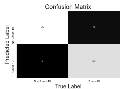
As we can see in the figure above, we have 5 errors on a total of 50 samples, where 2 predictions are Type II errors and 3 other predictions are Type I errors. So what does this mean? Is this good for our alternative hypothesis? does it negate \(H_0\) or confirms it? Can we conclude that the Covid 19 test is reliable?

This will be the topic of the next article.

To sum Up

This short article was an attempt to clarify the confusion often observed around the confusion matrix. We put the confusion matrix in the context of hypothesis testing. We also saw that in statistical hypothesis testing there are always two hypotheses competing against each other: a null hypothesis (\(H_0\)) and an alternative hypothesis (\(H_a\)). It is the alternative hypothesis that represents the research hypothesis and not the null hypothesis. We have also introduced the two kind of errors that could occur in the confusion matrix, and why it is important to differentiate between them. At the end, we run a small programming example using python and showed how easy it is to plot a confusion matrix using seaborn.