Customer Segmentation using RFM Analysis
Introduction
The field of marketing analytics is very broad and can include fascinating topics such as:
- Text mining,
- Social network analysis,
- sentiment analysis,
- realtime bidding and so on.
However, at the heart of marketing lie few basic questions, that often remain unanswered:
- Who are my customers?
- Which customers should I target, and spend most of my marketing budget on?
- What is the future value of my customers?
In this tutorial, we will explore the first two questions using customer segmentation techniques involving RFM analysis along with HCA.
Customer Segmentation
You can’t treat your customers the same way, offer them the same product, charge the same price, or communicate the same benefits. Otherwise you will miss a lot of value. So you need to understand the distinctions in your customers’ needs, wants, preferences and behaviors. Only then can you customize your offering, personalize your customer approach, and optimize your marketing campaigns.
Now, in today’s digital world, almost every online retailer holds a massive customer database. So, how do we deal with big customer databases?
Treating each and every customer individually is very costly. The answer is, of course, segmentation. I know, you’ve already guessed that yourselves.
A great segmentation is all about finding a good balance between simplifying enough, so it remains usable and not simplifying too much, so it’s still statistically and managerially relevant.
RFM Analysis
RFM (Recency, Frequency, Monetary) analysis is a segmentation approach based on customer behavior. It groups customers according to their purchasing history (How recently, how frequently, and how much has a customer spent on past purchases). It is one of the best predictor of future purchase and customer lifetime value in terms of their activity and engagement.
Recency indicates when a customer made his or her last purchase. Usually the smaller the recency, that is the more recent the last purchase, the more likely the next purchase will happen soon. On the other hand, if a customer has lapsed and has not made any purchase for a long period of time, he may have lost interest or switched to competition.
Frequency is about the number of customers purchases in a given period of time. Customers who bought frequently were more likely to buy again, as opposed to customers who made only one or two purchases.
Monetary is about how much a customer has spent in total during a given period. Customers who spend more should be treated differently than customers who spend less. Furthermore, they are more likely to buy again.
Practical Example in Python
We start by loading the required libraries and the dataset, and set up our programming environment. Also, make sure you have pandassql and squarify installed.
import numpy as np
import pandas as pd
import matplotlib.pyplot as plt
from pandasql import sqldf
from sklearn.preprocessing import scale
from scipy.spatial.distance import pdist
from scipy.cluster.hierarchy import dendrogram , linkage, cut_tree
import squarify
# Notebooks set up
pysqldf = lambda q: sqldf(q, globals())
%precision %.2f
pd.options.display.float_format = '{:,.2f}'.format
plt.rcParams["figure.figsize"] = (12,8)

# read the dataset from the csv file
headers = ['customer_id', 'purchase_amount', 'date_of_purchase']
df = pd.read_csv('../Datasets/purchases.txt', header=None,
                 names=headers, sep='\t')
Data Wrangling
The dataframe consists of 51,243 observations across 3 variables:
- Customer ID,
- purchase amount in USD and
- date of purchase
The data is clean and covers the period January 2nd 2005 to December 31st 2015.
df.info()
<class 'pandas.core.frame.DataFrame'>
RangeIndex: 51243 entries, 0 to 51242
Data columns (total 3 columns):
 #   Column            Non-Null Count  Dtype
---  ------            --------------  -----
 0   customer_id       51243 non-null  int64
 1   purchase_amount   51243 non-null  float64
 2   date_of_purchase  51243 non-null  object
dtypes: float64(1), int64(1), object(1)
memory usage: 1.2+ MB
We proceed by converting the data_of_purchase column from object to a date object.
# Transform the last column to a date object
df['date_of_purchase'] = pd.to_datetime(df['date_of_purchase'], format='%Y-%m-%d')
To calculate the recency, we create a new variable day_since that contains the number of days since the last purchase. To do this, we set January 1, 2016 as the start date and count the number of days since the last purchase for each customer backwards using the customers ID.
# Extract year of purchase and save it as a column
df['year_of_purchase'] = df['date_of_purchase'].dt.year
# Add a day_since column showing the difference between last purchase and a basedate
basedate = pd.Timestamp('2016-01-01')
df['days_since'] = (basedate - df['date_of_purchase']).dt.days
RFM Computation
To implement the RFM analysis, further data processing need to be done.
Next we are going to compute the customers recency, frequency and average purchase amount. This part is a bit tricky, particularly when implemented with pandas. The trick here is that the customer ID is unique for each customer. So even though we have 51,243 purchases, we will only have as many unique customer IDs as there are in the database.
For each customer, we now need to calculate the minimum number of days between all of their purchases and January 1, 2016. By taking the minimum number of days, we obviously have the day of the last purchase, which is the exact definition of recency.
The next step is to calculate the frequency for each customer, namely how many purchases this customer has made.
This is achieved with the python sql module:
# Compute recency, frequency, and average purchase amount
q = """
        SELECT customer_id,
        MIN(days_since) AS 'recency',
        COUNT(*) AS 'frequency',
        AVG(purchase_amount) AS 'amount'
        FROM df GROUP BY 1"""
customers = sqldf(q)
The asterisk here actually refers to anything in the data that is related to this customer; and then for the amount, we averaged the purchase amount for that specific customer ID and named that aggregate calculation as amount.
Now, the trick is we want to make sure that each row only appears once per customer. So we’re going to calculate that from the data and group by one, which means that everything here is going to be calculated and grouped by customer ID.
Sure, it would have been possible to do all the computations with pandas only. However, this would have required much more work. When working with databases, SQL knowledge is an advantage. Indeed, a single sql command is all that is needed to create an RFM table.
The results are then stored under the variable customers and the first five entries have the following values:
customers.head()
+----+---------------+-----------+-------------+----------+
|    |   customer_id |   recency |   frequency |   amount |
|----+---------------+-----------+-------------+----------|
|  0 |            10 |      3829 |           1 |       30 |
|  1 |            80 |       343 |           7 |  71.4286 |
|  2 |            90 |       758 |          10 |    115.8 |
|  3 |           120 |      1401 |           1 |       20 |
|  4 |           130 |      2970 |           2 |       50 |
+----+---------------+-----------+-------------+----------+
Exploratory Data Analysis
We start by generating some descriptive statistics, including those that summarize the central tendency, dispersion and shape of each of our RFM variables.
customers[['recency', 'frequency', 'amount']].describe()
+-------+-----------+-------------+----------+
|       |   recency |   frequency |   amount |
|-------+-----------+-------------+----------|
| count |     18417 |       18417 |    18417 |
| mean  |   1253.04 |     2.78237 |   57.793 |
| std   |   1081.44 |     2.93689 |   154.36 |
| min   |         1 |           1 |        5 |
| 25%   |       244 |           1 |  21.6667 |
| 50%   |      1070 |           2 |       30 |
| 75%   |      2130 |           3 |       50 |
| max   |      4014 |          45 |     4500 |
+-------+-----------+-------------+----------+
Then we plot the distributions of the RFM variables.
# Plot the recency distribution
plt.style.use('seaborn-whitegrid')
customers.hist(column='recency', bins=31)
plt.ylabel('Customers', fontsize=15)
plt.xlabel('Days Since Last Purchase', fontsize=15)
plt.xlim(0,);
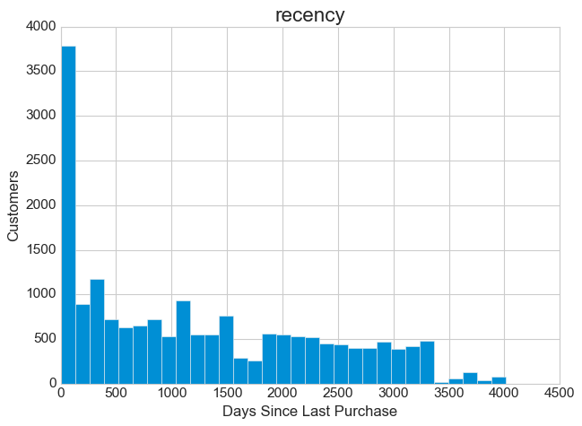
Except for a peak on the very left, the recency distribution is relatively uniform. This is good to see, because it means that our business has been gaining attention lately and has been generating record sales. It’s always worth doing a detailed analysis when it comes to outliers or exceptions. So I recommend taking a closer look at this peak to determine its triggers and drivers. It could be that our last marketing campaign was a success or that the pop-up sale we had recently was the consequence. So try to figure out the reason for this and take advantage of it.
# Plot the frequency distribution
customers.hist(column='frequency', bins=41)
plt.ylabel('Customers', fontsize=15)
plt.xlabel('Number of Purchases', fontsize=15)
plt.xlim(0,20);
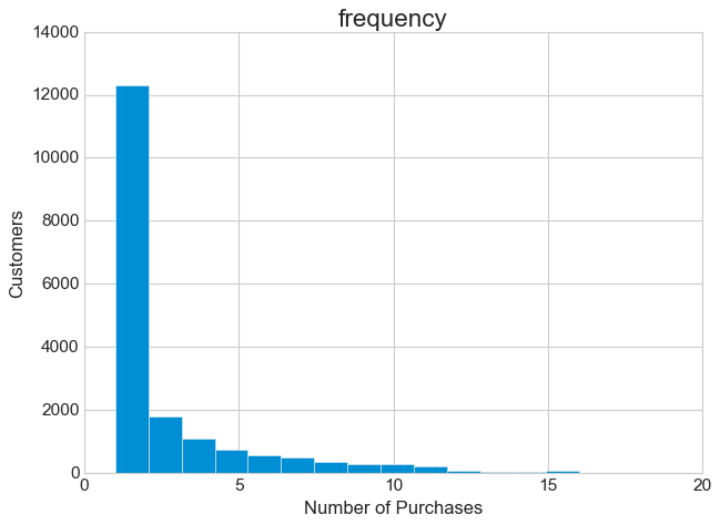
The frequency distribution is extremely skewed to the right. Almost 50% of all customers have only made one purchase. Again, further clarification is necessary here. It is possible that most one-time purchases are recent, first-time transactions. And with a marketing approach tailored to the relevant customer segments, we could encourage these customers to make their next purchase.
customers.hist(column='amount', bins=601)
plt.ylabel('Customers', fontsize=15)
plt.xlabel('Average Amount in $', fontsize=15)
plt.xlim(0,400)
plt.ylim(0,);
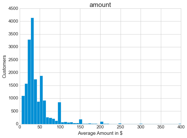
Due to the presence of some extreme outliers, it is preferable to use the median here. 50% of all transactions are between $5 and $30.
This was a small overview of how to conduct an exploratory data analysis. Usually, at this stage of analysis, we develop hypotheses that we want to test later, especially with respect to ambiguous relationships such as finding out if it involves correlation or causation. Therefore, it is best to spend a little more time exploring your dataset.
Lets now move on to customer segmentation.
Hierarchical Cluster Analysis
Before starting the data transformation it is better to keep a copy of the original data, in case something goes wrong.
# Copy the dataset
new_data = customers.copy()
new_data.set_index('customer_id', inplace=True)
Data preprocessing is an essential part of segmentation and ML algorithms in general. We need to prepare and transform our data, so the segmentation variables can be compared to one another.
Since our segmentation variables don’t use the same scales, we need to standardize them. In statistics, standardization means to subtract the mean and divide by the standard deviation:
\[Standardize=\frac{Data - data~mean}{Data~standard~deviation}\]Regardless of what the original scale was, days, dollars, or number of purchases, they can now be related to one another.
Another problem to deal with is the dispersion or skewness of data. Skewness indicates the direction and relative magnitude of a distribution’s deviation from the normal distribution. In the figure above, we see that the average purchase amount in $ is right skewed, meaning that there is a minority of very large positive values. And when data is extremely skewed, it may not be adequate for segmentation. In such a situation, it can be useful to convert it to a logarithmic scale.
# transform amount into a logarithmic scale and plot the result
new_data['amount'] = np.log10(new_data['amount'])
# plot
ax, fig = plt.subplots()
new_data['amount'].plot(kind='hist', density=True, bins=40)
new_data['amount'].plot(kind='kde')

plt.xlim(0,4)
plt.ylim(0,);
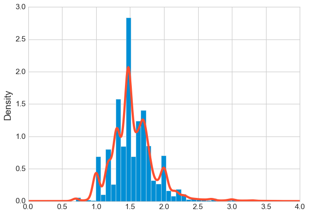
From the plot above we can see that after the transformation our data became more symmetrical and less skewed.
Now we scale our data to ensure that the clustering algorithm is stable against outliers and extreme values. Not all machine learning algorithms require feature scaling. However, for distance-based algorithms such as HCA, KNN, K-means, or SVM, scaling is required. The reason is that all these algorithms use distances between data points to determine similarities.
# Now we scale our data and we save it as dataframe:
new_data = pd.DataFrame(scale(new_data), index=new_data.index,
                        columns=new_data.columns)
# computing the distance would generate a huge matrix:
print(f'Dimension of the distance matrix: ({new_data.shape[0]**2}, {new_data.shape[1]})')
Dimension of the distance matrix: (339185889, 3)
Calculating the distance matrix would generate a huge matrix. Therefore, we take a sample from our RFM dataset with a sampling rate of 10%. It means that only every 10th customer is considered in our segmentation.
# Since the distance matrix is that huge,
# we are sampling with a sampling rate of 10%
sample = np.arange(0, 18417, 10)
sample[:10]
array([ 0, 10, 20, 30, 40, 50, 60, 70, 80, 90])
Let’s display some random samples from our newly generated dataframe; the one we will use to perform hierarchical clustering.
new_data_sample = new_data.iloc[sample]
new_data_sample.sample(5)
+---------------+-----------+-------------+----------+
|   customer_id |   recency |   frequency |   amount |
|---------------+-----------+-------------+----------|
|         69760 |      3178 |           1 |  1.47712 |
|        147990 |      1911 |           1 |  1.30103 |
|        100510 |      2739 |           1 |  1.47712 |
|        138990 |        22 |           9 |  1.74473 |
|        258230 |        55 |           1 |        2 |
+---------------+-----------+-------------+----------+
customers_sample = customers.iloc[sample].copy()
# we compute the distances on the sampled data
d = pdist(new_data_sample) # default metric is euclidean
# and we perform the hierarchical clustering:
hcward = linkage(d, method='ward')
pdist() computes pairwise distances between observations. The default distance metric is Euclidean. There are, however, many other metrics to choose from, such as: minkowski, chebyshev and hamming. Here we choose the default method.
The clustering is performed by calling the linkage() using the ward method. There are many other methods to choose from and it doesn’t have to be ward.
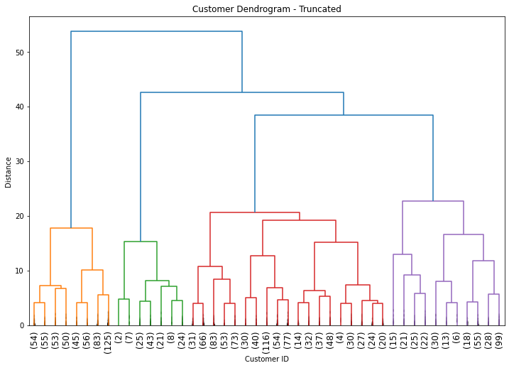
After performing HCA we display the results using dendrogram.
# Plot dendrogram
plt.title("Customer Dendrogram - Truncated")
dend = dendrogram(hcward,
                  truncate_mode='lastp',
                  p = 45,
                  show_contracted=True,
                  leaf_rotation=90,
                  leaf_font_size=12);
plt.xlabel('Customer ID')
plt.ylabel('Distance');
Determining the Number of Clusters
In RFM models it is usual to choose 11 clusters as recommended by PULTER and other experts. They also provide a well-documented customer segment table with the description of each segment as well as a list of marketing actions corresponding to each segment.
However, it is not necessary to have 11 clusters.
From the dendrogram we can see that 4 clusters make sense for this scenario as well as for simplicity sake. So let’s try that.
Remember: When it comes to cut-off selection there is no golden method on how to pick the perfect number of clusters. What matters is to use the right clustering approach for the business problem at hand and that your conclusions are actionable.
# Cut at 4 clusters
members = cut_tree(hcward, n_clusters=4)
# Assign to each customer a group
groups, counts = np.unique(members, return_counts=True)
segments = dict(zip(groups, counts))

customers_sample['group'] = members.flatten()
# Create a table with the obtained groups and their characteristics
clusters = customers_sample[['recency', 'frequency', 'amount', 'group']].groupby('group').mean()
clusters
+---------+-----------+-------------+----------+
|   group |   recency |   frequency |   amount |
|---------+-----------+-------------+----------|
|       0 |   2612.50 |        1.30 |    29.03 |
|       1 |    193.65 |       10.62 |    42.02 |
|       2 |    712.52 |        2.55 |    31.12 |
|       3 |    972.55 |        2.76 |   149.70 |
+---------+-----------+-------------+----------+
print(f'Number of customers per segment: {segments}')
Number of customers per segment: {0: 521, 1: 130, 2: 859, 3: 332}
Clusters Profiling
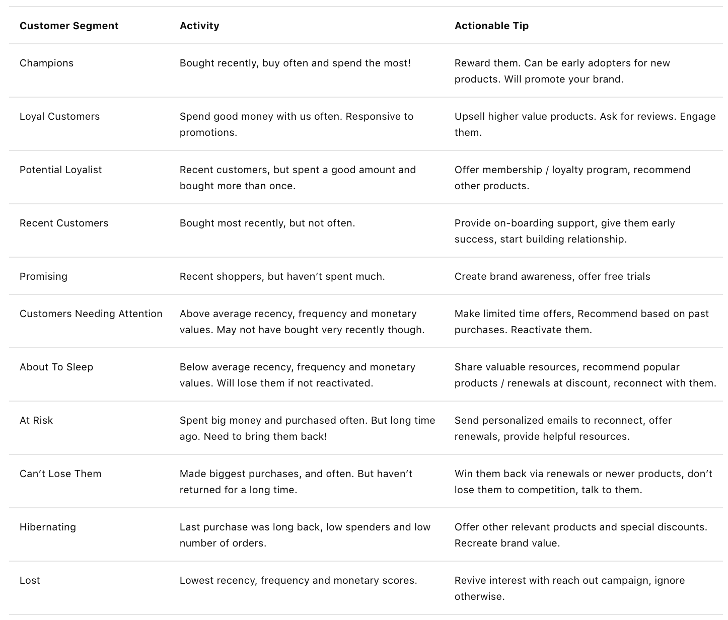
Now that we have our clusters and are convinced of their number, we can start profiling them. For this purpose we are going to use the Customer Segments table from putler.
- Group 0 has the lowest recency, frequency and monetary value. Therefore, we refer to this group as Lost. You’d better ignore it completely.
- Group 1 consists of your Loyal Customers. They buy often and spend a good money with us. As actionable tips I would suggest to Offer them higher value products, ask for reviews and create meaningful interactions with them, using engagement marketing strategies.
- Group 2 are the Customers Needing Attention. It’s by far your largest group, so you need to reconnect with the customers in this group. The sooner, the better; before they fall into the group “about to sleep”. You might, for instance, offer them limited-time product deals based on their past purchases.
- Group 3 contains the Can’t Lose Them customers. They spent the most money in our business, but haven’t come back for a long time. Win them back, talk to them, and don’t lose them to your competitors. Try to reengage them with your company through renewals or new products, or perhaps special marketing events.
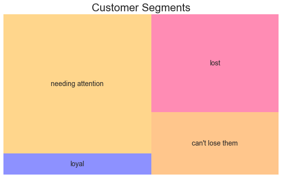
Let us include the profiling results in our clusters variable and create an appealing visualization of the findings. After all, it is your job as a business analyst to convince the management team to implement your recommendations for action.
clusters['n_customers'] = customers_sample['group'].value_counts()
clusters['cluster_names'] = ['lost', 'loyal', 'needing attention', "can't lose them"]

# Visualization
plt.set_cmap('hsv')
clusters.sort_values(by=['recency', 'amount'], ascending=[True, False], inplace=True)

squarify.plot(sizes=clusters['n_customers'],
              label=clusters['cluster_names'], alpha=.45 )
plt.title("RFM Segments",fontsize=22)
plt.axis('off');
Summary
In this tutorial, we presented another use case of hierarchical clustering: Customer Segmentation based on buying behavior. It is a simple yet powerful technique when it comes to customer targeting and precision marketing.
We also showed how clusters profiling works and how you can tailor your marketing campaigns to the customer segments whose expected profitability exceeds the cost to reaching them. However, this segmentation method is not without problems and comes with a number of limitations:
- New customers are constantly being added to the database, which requires frequent updating of the segmentation model.
- Clusters can capture seasonal customers buying behaviors, so results are no longer generalizable to different time periods.
- Frequent updates can be expensive. Unless they are automated and you don’t need each time to hire a data scientist.
This is the main reason why companies are still reluctant to use statistical segmentation and prefer to rely on managerial segmentation.
Non-statistical segmentation approaches are based on simple rules and guidelines and rely heavily on subjective judgment. This also comes with some drawbacks, as it can be severely affected by various types of biases and cognitive limitations when processing complex data.
Which one you choose depends on your goals and budget. However, if you prefer the latter approach, I strongly recommend that you perform statistical segmentation, at least once as exploratory tool, to identify complex patterns in multivariate data sets. Then you can set up your segmentation rules around them.
References
- Karl Melo. Customer Analytics I - Customer Segmentation. 2016
- Navlani, A. Introduction to Customer Segmentation in Python. datacamp, 2018.
- Lilien, Gary L, Arvind Rangaswamy, and Arnaud De Bruyn. 2017. Principles of Marketing Engineering and Analytics. State College, PA: Decisionpro.
- Jim Novo. Turning Customer Data into Profits
- Anish Nair. RFM Analysis For Successful Customer Segmentation. putler, 2022.
- Kohavi, Ron, Llew Mason, Rajesh Parekh, and Zijian Zheng. 2004. “Lessons and Challenges from Mining Retail E-Commerce Data.” Machine Learning 57 (1/2): 83–113.
- Dataset from Github repo. Accessed 25 October 2021.
Business Analytics Tutorial Hierarchical Cluster Analysis Customer Segmentation 