Customer Segmentation and Profiling: A Managerial Approach

Introduction

One of the most used and familiar concepts in marketing is market segmentation, that is, the division of markets, based on common characteristics such as geographic, demographic, psychographic and behavioristic, into homogeneous groups of customers, in order to develop segment-specific marketing strategies or to look for new product opportunities to effectively capture the target segments.

In reality, there is no single best method for segmenting a market and, more importantly, the way we segment a market should reflect what we intend to achieve. Useful segments must, however, possess the following four qualities [4]:

1. Measurability; in terms of the size and purchasing power of the segment.
2. Actionability, that is, the extent to which it is possible to design an effective marketing plan for the target segment
3. Accessibility which means that your company’s marketing activities and distribution system are capable of reaching and adequately serving the target segment.
4. Substantiality; implying that the target segments are large enough to be profitable.

Broadly speaking, any market segmentation falls into one of the following two approaches: a priori (or prescriptive) and post hoc (or exploratory) segmentation. Segmentation based on hierarchical cluster analysis, which we introduced in the last tutorial, is a typical example of exploratory post-hoc segmentation. In this tutorial, we will introduce and implement an a priori approach to segmentation, namely managerial market segmentation.

Managerial Segmentation

Managerial segmentation is an a priori segmentation, and is performed when the manager proactively chooses the basis of the market analysis and the variables to be included in the segmentation. Hence, the basis for segmentation varies depending on the specific business decisions that management is facing. For instance, if the management is concerned with the likely impact of a price increase on the customers, the appropriate basis might be the current customers’ price sensitivity. If, however the management is concerned with the loss of customers, the basis for segmentation could be recency.

In this tutorial, we want to predict which customers are most likely to make further purchases in the near future. A basic criterion for this would be whether the customer has made a purchase recently or not. After all, someone who bought at our store a few weeks ago is much more likely to buy again in the future than someone whose last purchase was several years ago.
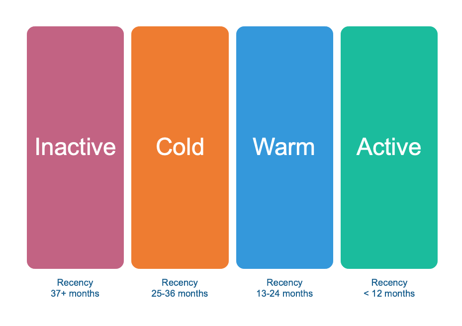
In this case, an appropriate model would be to divide our customer database into four groups or segments based on recency; where:

1. Active are customers whose last purchase was within the last 12 months.
2. Warm if their last purchase was one year ago, that is, between 13 and 24 months.
3. Cold those whose last purchase was between 25 and 36 months ago; and
4. Those who have not bought anything from us for more than 3 years, we call Inactive.

Now, given the scope and diversity of marketing decisions, attempting to use a single basis for segmentation to develop a marketing strategy is likely to result in adopting the wrong solutions and wasting resources. So let’s add another variable to our segmentation model, namely average spending. By doing so, we want to differentiate between valuable and less valuable customers in each subgroup within Warm and Active customers. Furthermore, we want to differentiate between those who have only made one purchase so far, regardless of how much money they spend, and refer to them as New Customers. That is an RFM analysis.

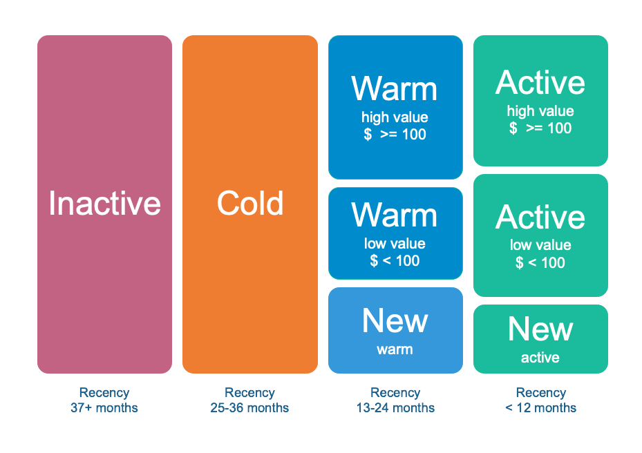
As a result, we end up with a total of eight segments. At this point, we can decide which groups to allocate our marketing budget to and how to target our marketing campaigns towards them.

Customer Profiling

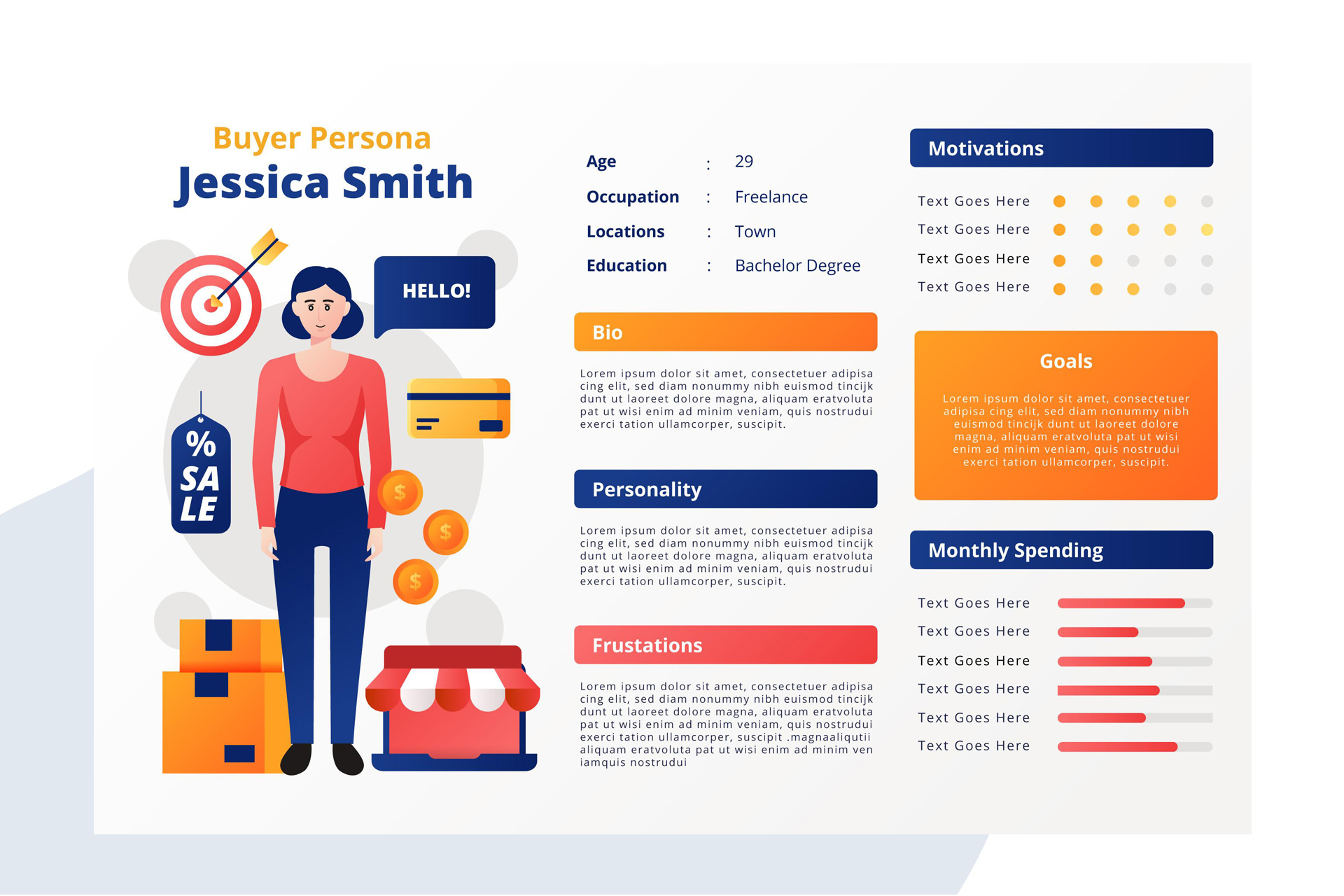
Once we are done with the segmentation, we want to describe each segment in more detail. This is best done by creating a semi-fictional archetype from the average profile of all customers in a segment so that it personifies the key characteristics of those customers. Don’t stop there, I recommend to give it a suitable name and even invent a little narrative about it. This is also known as Buyer Persona or Centroid ¹.

Practical Example in Python

Now that we are done with the theory, let’s have some fun. In the following we want to implement the height market segment depicted above. We will be using the same data as in the previous tutorial. It consists of 51,243 observations across 3 variables:

1. Customer ID,
2. purchase amount in USD and
3. date of purchase

The data includes all sales that occurred between January 2, 2005 and December 31, 2015. The dataset is tidy and no records are missing.
Having imported the necessary Python libraries, the next step is to load the data as Panda’s dataframe and check that everything is fine.

# Load the required libraries
import numpy as np
import pandas as pd
import matplotlib.pyplot as plt
from pandasql import sqldf
from tabulate import tabulate

# Set up the jupyter lab environment
%precision %.2f
pd.options.display.float_format = '{:,.2f}'.format
plt.rcParams["figure.figsize"] = (12,8)

It is also recommended to replace the names of the variables with meaningful and easy-to-remember names.

columns = ['customer_id', 'purchase_amount', 'date_of_purchase']
df = pd.read_csv('purchases.txt', header=None, sep='\t',
            names=columns)
df.sample(n=5, random_state=57)

+-------+---------------+-------------------+--------------------+
|       |   customer_id |   purchase_amount | date_of_purchase   |
|-------+---------------+-------------------+--------------------|
|  4510 |          8060 |                30 | 2014-12-24         |
| 17761 |        109180 |                50 | 2009-11-25         |
| 39110 |          9830 |                30 | 2007-06-12         |
| 37183 |         56400 |                60 | 2009-09-30         |
| 33705 |         41290 |                60 | 2007-08-21         |
+-------+---------------+-------------------+--------------------+

We proceed by converting data_of_purchase to a datetime object and save the year of purchase as a new variable. We also calculate the days elapsed since the last purchase and January 1, 2016; which we consider to be the most recent date and then print the results.

# interpret the last column as datetime
df['date_of_purchase'] = pd.to_datetime(df['date_of_purchase'], 
                                        format='%Y-%m-%d')
# Extract year of purchase and save it as a column
df['year_of_purchase'] = df['date_of_purchase'].dt.year
# Add a day_since column showing the difference between last purchase and a basedate
basedate = pd.Timestamp('2016-01-01')
df['days_since'] = (basedate - df['date_of_purchase']).dt.days
# print dataframe info
df.info()

<class 'pandas.core.frame.DataFrame'>
RangeIndex: 51243 entries, 0 to 51242
Data columns (total 5 columns):
 #   Column            Non-Null Count  Dtype         
---  ------            --------------  -----         
 0   customer_id       51243 non-null  int64         
 1   purchase_amount   51243 non-null  float64       
 2   date_of_purchase  51243 non-null  datetime64[ns]
 3   year_of_purchase  51243 non-null  int64         
 4   days_since        51243 non-null  int64         
dtypes: datetime64[ns](1), float64(1), int64(3)
memory usage: 2.0 MB

Everything looks good. So let’s get on with the RFM analysis.

RFM Analysis

Now we want to compute the customers recency, frequency and average purchase amount. This part is done using SQL queries from pandasql library. The library uses SQLite syntax and can execute complex SQL queries. This keeps our code neat, comprehensible and easy to debug.

# Compute recency, frequency, and average purchase amount
q = """
        SELECT customer_id,
        MIN(days_since) AS 'recency',
        COUNT(*) AS 'frequency',
        AVG(purchase_amount) AS 'amount'
        FROM df GROUP BY 1"""
customers = sqldf(q)

Nothing we have implemented so far is new. We have already seen the same code in the previous tutorial. So if you have trouble following, especially when it comes to SQL, I recommend you take a look at the first part of the practical example from Customer Segmentation using RFM Analysis.
As result we get around 18,000 customers and four variables: customer_id, recency, frequency and amount.

Let’s print some descriptive statistics as well as the first five rows of our RFM analysis.

print(tabulate(customers_2015.describe(), headers='keys', tablefmt='psql'))

+-------+---------------+-----------+------------------+-------------+------------+
|       |   customer_id |   recency |   first_purchase |   frequency |     amount |
|-------+---------------+-----------+------------------+-------------+------------|
| count |       18417   |  18417    |         18417    | 18417       | 18417      |
| mean  |      137574   |   1253.04 |          1984.01 |     2.78237 |    57.793  |
| std   |       69504.6 |   1081.44 |          1133.41 |     2.93689 |   154.36   |
| min   |          10   |      1    |             1    |     1       |     5      |
| 25%   |       81990   |    244    |           988    |     1       |    21.6667 |
| 50%   |      136430   |   1070    |          2087    |     2       |    30      |
| 75%   |      195100   |   2130    |          2992    |     3       |    50      |
| max   |      264200   |   4014    |          4016    |    45       |  4500      |
+-------+---------------+-----------+------------------+-------------+------------+

print(tabulate(customers.head() , headers='keys', tablefmt='psql'))

+----+---------------+-----------+------------------+-------------+----------+
|    |   customer_id |   recency |   first_purchase |   frequency |   amount |
|----+---------------+-----------+------------------+-------------+----------|
|  0 |            10 |      3829 |             3829 |           1 |  30      |
|  1 |            80 |       343 |             3751 |           7 |  71.4286 |
|  2 |            90 |       758 |             3783 |          10 | 115.8    |
|  3 |           120 |      1401 |             1401 |           1 |  20      |
|  4 |           130 |      2970 |             3710 |           2 |  50      |
+----+---------------+-----------+------------------+-------------+----------+

And as they say, a picture is worth a thousand words:

customers.iloc[:,1:].hist(bins=30, figsize=(15, 10));

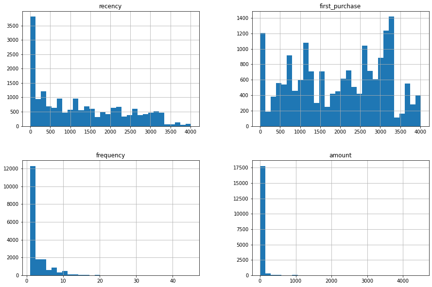
In the next section we will implement the first segmentation model based on recency. On the basis of this model, we will later build the more complex eight-segment model.

Managerial Segmentation Based on One Variable

Instead of using machine learning to identify segments as seen in the previous tutorial, we will now implement a managerial segmentation. Simply put, it is nothing more but a sequence of if-then-else statements and consists of four segments in total: active, warm, cold and inactive.

We first begin by identifying the segment of inactive customers. According to the above definition, these are those who have not made a single purchase in more than three years:

customers.loc[customers['recency'] > 365*3, 'segment'] = 'inactive'
# Fill missing values with NA/NaN values
customers['segment'] =  customers['segment'].fillna('NA')
customers_2015['segment'].value_counts()

NA          9259
inactive    9158
Name: segment, dtype: int64

So nearly half of our customers are inactive. This is not good, as we know an inactive customer is a lost customer. Now, before we try to recover lost customers, we first need to understand the reasons behind our customers’ attrition. This, in turn, requires us to dive deeper into our data, to benchmark against our competitors, and also to send out customer loss surveys to the relevant customers. As we gain a better understanding of the reasons, we can implement a marketing strategy aimed at recovering high-value customers.

The rest of the customers are then mapped to the corresponding segments using the same approach.

# Build the Cold segment
customers.loc[(customers['recency']<= 365*3) & 
                   (customers['recency'] > 356*2), 'segment'] = "cold"
# Warm Segment
customers.loc[(customers['recency']<= 365*2) & 
                   (customers['recency'] > 365*1), 'segment'] = "warm"
# Active segment
customers.loc[customers['recency']<= 365, 'segment'] = "active"

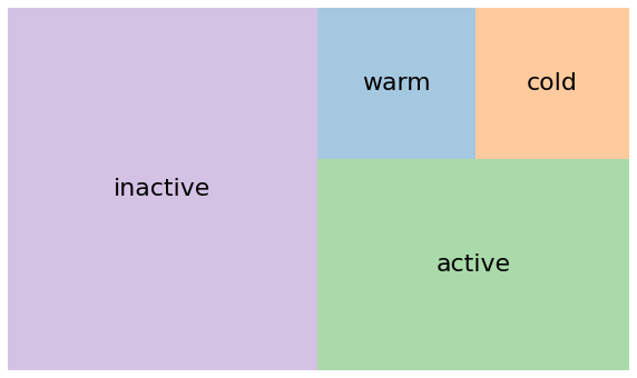
Let’s print and visualize the results. Make sure before that you have the squarify package installed. It is very handy, when it comes to Tremapping ².

# Print the results
clusters = customers['segment'].value_counts()
clusters

inactive    9158
active      5398
warm        1958
cold        1903
Name: segment, dtype: int64

plt.rcParams["figure.figsize"] = (10,6)
plt.rcParams.update({'font.size': 22})


squarify.plot(sizes=clusters, 
              label=clusters.index, 
              color=['tab:purple', 'tab:green', 'tab:blue', 'tab:orange'], alpha=.4 )
plt.axis('off');

Managerial Segmentation Based on RFM

In this section, we will add two new variables to the segmentation model from above, which are: frequency and monetary. More specifically, we want to separate new customers from the rest of the customers and differentiate between high and low value customers. To increase efficiency, we want to limit our marketing activities to just the following two market segments: active and warm.

We begin by adding a new group to the warm segment: new warm, which refers to those who have made only a single purchase in the past two years. Then, we divide the warm segment into two subgroups based on how much money they spend on average, with $100 as the threshold.

# Further segmentation of the warm segment:
customers.loc[(customers['segment'] == "warm") &
                  (customers['first_purchase'] <= 365*2), 'segment'] = "new warm"

customers.loc[(customers['segment'] == "warm") &
                  (customers['amount'] < 100), 'segment'] = "warm low value"

customers.loc[(customers['segment'] == "warm") &
                  (customers['amount'] >= 100), 'segment'] = "warm high value"

Finally, we do the same for our Active segment.

customers.loc[(customers['segment'] == "active") &
                  (customers['first_purchase'] <= 365), 'segment'] = "new active"

customers.loc[(customers['segment'] == "active") &
                  (customers['amount'] < 100), 'segment'] = "active low value"

customers.loc[(customers['segment'] == "active") &
                  (customers['amount'] >= 100), 'segment'] = "active high value"

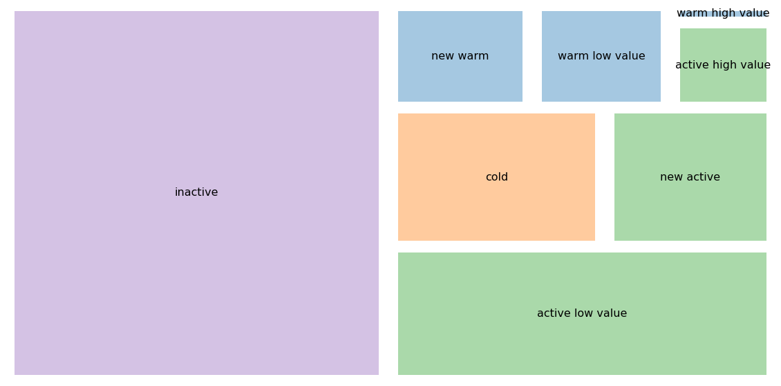
As output we get:

customers['segment'].value_counts()

inactive             9158
active low value     3313
cold                 1903
new active           1512
new warm              938
warm low value        901
active high value     573
warm high value       119
Name: segment, dtype: int64

To make the results look better, let’s arrange the segments in the order shown above and print the first five and last five entries in our Pandas dataframe.

# We start first by changing the type of the segment variable to categorical
customers['segment'] = customers['segment'].astype('category')
customers['segment_sort'] = pd.Categorical( customers['segment'],
        categories=['inactive', 'cold', 'warm high value','warm low value', 
           'new warm', 'active high value', 'active low value',
           'new active'], ordered=True)
customers.sort_values('segment_sort', inplace=True)

# print first 5 rows
print(tabulate(customers[['customer_id', 'segment_sort']].head(), headers='keys', 
               tablefmt='psql', showindex=False))

+---------------+----------------+
|   customer_id | segment_sort   |
|---------------+----------------|
|            10 | inactive       |
|        119690 | inactive       |
|        119710 | inactive       |
|        119720 | inactive       |
|        119730 | inactive       |
+---------------+----------------+

# print the last 5 rows
print(tabulate(customers_2015[['customer_id', 'segment_sort']].tail(), headers='keys', 
               tablefmt='psql', showindex=False))

+---------------+----------------+
|   customer_id | segment_sort   |
|---------------+----------------|
|        252380 | new active     |
|        252370 | new active     |
|        252360 | new active     |
|        252450 | new active     |
|        264200 | new active     |
+---------------+----------------+

If you like, we can plot the results as a treemap again to give you a sense on how the segment sizes compare to each other.

plt.rcParams["figure.figsize"] = (20,10)
plt.rcParams.update({'font.size': 16})

colors = ['tab:purple', 'tab:green', 'tab:orange', 'tab:green', 
                     'tab:blue', 'tab:blue', 'tab:green', 'tab:blue']
squarify.plot(sizes=clusters, 
              label=clusters.index, 
              color=colors, pad=True, alpha=.4,
              norm_x=80, norm_y=65)
plt.axis('off');

Alright. Now we want to create buyer personas for the target segments so we can develop the right marketing activities for each segment to increase sales and reduce customer churn. Unfortunately, we will not cover these topics here. If you are interested in how it works, check out my previous tutorial.

Summary

Managerial segmentation is basically a sequence of if-then statements based on simple rules. The defined segments need, however to be relevant to the management using the segmentation. Thus, it relies heavily on the experience and subjective judgment of the manager in charge and usually leads to the implementation of familiar strategies. Now, applying known segmentation models too early without exploring new ones can lead to inferior results. Ideally, is to find a balance between exploring new strategies and applying known ones. After all, to adapt to complex and rapidly changing business environments, managers need to explore and refine new knowledge. This is also known as exploration-exploitation dilemma in cognitive science and ambidexterity in management theory. Even more problematic is the fact that managers are usually older. So, are they still capable of innovating and thinking outside the box?³
You tell me.

References

1. Lilien, Gary L, Arvind Rangaswamy, and Arnaud De Bruyn. 2017. Principles of Marketing Engineering and Analytics. State College, PA: Decisionpro.
2. Piercy, Nigel F., and Neil A. Morgan. 1993. “Strategic and Operational Market Segmentation: A Managerial Analysis.” Journal of Strategic Marketing 1 (2): 123–40. https://doi.org/10.1080/09652549300000008.
3. Wind, Yoram. 1978. “Issues and Advances in Segmentation Research.” Journal of Marketing Research 15 (3): 317. https://doi.org/10.2307/3150580.
4. Armstrong, G.M., S. Adam, S.M. Denize, M. Volkov, and P. Kotler. 2017. Principles of Marketing. Pearson Australia. https://books.google.cd/books?id=KndhuwEACAAJ.
5. Laureiro-Martínez, Daniella, Stefano Brusoni, Nicola Canessa, and Maurizio Zollo. 2015. “Understanding the Exploration-Exploitation Dilemma: An FMRI Study of Attention Control and Decision-Making Performance: Understanding the Exploration-Exploitation Dilemma.” Strategic Management Journal 36 (3): 319–38. https://doi.org/10.1002/smj.2221.
6. Arnaud De Bruyn. Foundations of marketing analytics (MOOC). Coursera.
7. Dataset from Github repo. Accessed 15 December 2021.