From RFM Analysis to Predictive Scoring Models
Introduction
Business forecasting is not about accurately predicting the future, nor is it an end in itself. It is a means to help companies manage uncertainty and develop strategies to minimize potential risks and threats or maximize financial returns. It relies on identifying and estimating past patterns that are then generalized to forecast the future. As such, forecasting has a wide range of business applications and can be useful throughout the value chain of any organization.
For instance, forecasting customer purchases allows companies not only to calculate the expected revenue of each segment so they can focus on profitable ones, but also to properly plan inventory and manpower for the next period. Other business forecasting applications include customer lifetime value, credit card attrition or future revenues. In other words, every business needs forecasting.
In this tutorial we will develop a typical marketing application. We will predict the likelihood that a customer will make a purchase in a near future. And if so, we also want to predict how much s/he will spend. For this, we will first segment our customer database using RFM analysis –I hope you are by now familiar with this segmentation method– and then we will build two distinct models:
- A first model to calculate the probability of purchase
- A second model to predict the amount spent
For simplicity sake, we will use linear regression in both models. As it is one of the simplest supervised learning algorithms.
Finally, we will combine the two models into one large scoring model.
RFM Analysis and Customer Segmentation
In this section we will use the same code as in the previous tutorial. The only difference is that we will save the resulting customer segmentation as customers_2015 rather than just customers.
As usual, we start by importing the necessary libraries, setting up the notebook environment and reading the data set as a dataframe.
# import needed packages
import matplotlib as mpl
import matplotlib.pyplot as plt
import numpy as np
import pandas as pd
import patsy
import squarify
import statsmodels.api as sm
from pandasql import sqldf
from tabulate import tabulate

# Set up the notebook environment
pysqldf = lambda q: sqldf(q, globals())
%precision %.2f
pd.options.display.float_format = "{:,.2f}".format
plt.rcParams["figure.figsize"] = 10, 8

# Load text file into a local variable
columns = ["customer_id", "purchase_amount", "date_of_purchase"]
df = pd.read_csv("purchases.txt", header=None, sep="\t", names=columns)

# interpret the last column as datetime
df["date_of_purchase"] = pd.to_datetime(df["date_of_purchase"], format="%Y-%m-%d")
Then we add two variables: year_of_purchase and days_since.
# Extract year of purchase and save it as a column
df["year_of_purchase"] = df["date_of_purchase"].dt.year

# Add a day_since column showing the difference between last purchase and a basedate
basedate = pd.Timestamp("2016-01-01")
df["days_since"] = (basedate - df["date_of_purchase"]).dt.days
We now use SQL for the RFM analysis and then segment our customer database accordingly.
q = """
        SELECT customer_id,
        MIN(days_since) AS 'recency',
        MAX(days_since) AS 'first_purchase',
        COUNT(*) AS 'frequency',
        AVG(purchase_amount) AS 'amount'
        FROM df GROUP BY 1"""
customers_2015 = sqldf(q)
# Managerial Segmentation based on RFM analysis
customers_2015.loc[customers_2015["recency"] > 365 * 3, "segment"] = "inactive"
customers_2015["segment"] = customers_2015["segment"].fillna("NA")
customers_2015.loc[
    (customers_2015["recency"] <= 365 * 3) & (customers_2015["recency"] > 356 * 2),
    "segment",
] = "cold"
customers_2015.loc[
    (customers_2015["recency"] <= 365 * 2) & (customers_2015["recency"] > 365 * 1),
    "segment",
] = "warm"
customers_2015.loc[customers_2015["recency"] <= 365, "segment"] = "active"
customers_2015.loc[
    (customers_2015["segment"] == "warm")
    & (customers_2015["first_purchase"] <= 365 * 2),
    "segment",
] = "new warm"
customers_2015.loc[
    (customers_2015["segment"] == "warm") & (customers_2015["amount"] < 100), "segment"
] = "warm low value"
customers_2015.loc[
    (customers_2015["segment"] == "warm") & (customers_2015["amount"] >= 100), "segment"
] = "warm high value"
customers_2015.loc[
    (customers_2015["segment"] == "active") & (customers_2015["first_purchase"] <= 365),
    "segment",
] = "new active"
customers_2015.loc[
    (customers_2015["segment"] == "active") & (customers_2015["amount"] < 100),
    "segment",
] = "active low value"
customers_2015.loc[
    (customers_2015["segment"] == "active") & (customers_2015["amount"] >= 100),
    "segment",
] = "active high value"
Once we have the segments populated with corresponding customers we transform the type of the segment variable to categorical and reorder the segments, so that it makes more sense.
# Transform segment column datatype from object to category
customers_2015["segment"] = customers_2015["segment"].astype("category")
# Re-order segments in a better readable way
sorter = [
    "inactive",
    "cold",
    "warm high value",
    "warm low value",
    "new warm",
    "active high value",
    "active low value",
    "new active",
]
customers_2015.segment.cat.set_categories(sorter, inplace=True)
customers_2015.sort_values(["segment"], inplace=True)
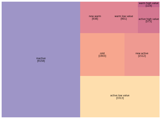
So let’s plot the results as a treemap using squarify.
plt.rcParams["figure.figsize"] = 12, 9
c2015 = pd.DataFrame(customers_2015["segment"].value_counts())
norm = mpl.colors.Normalize(vmin=min(c2015["segment"]), vmax=max(c2015["segment"]))
colors = [mpl.cm.RdYlBu_r(norm(value)) for value in c2015["segment"]]
squarify.plot(sizes=c2015["segment"], label=c2015.index,
              value=c2015.values, color=colors, alpha=0.6)
plt.axis("off");
We will also need to compute the revenue of each customer in 2015 to be able to predict the amount of the next purchase.
# Compute revenues generated by customers in 2015 using SQL
q = """
        SELECT customer_id,
        SUM(purchase_amount) AS 'revenue_2015'
        FROM df
        WHERE year_of_purchase = 2015
        GROUP BY 1
    """
revenue_2015 = sqldf(q)
Note that not all customers have made a purchase in 2015.
print('Number of customers with at least one completed payment:', revenue_2015.shape[0])
print('Total number of customers as in 2015:', customers_2015.shape[0])
Number of customers with at least one completed payment: 5398
Total number of customers as in 2015: 18417
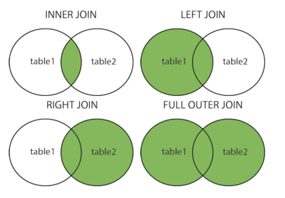
revenue_2015 contains only 5,398 observations, while we have 18,417 customers to date. This is because a large portion of our customers were actually inactive in 2015. Nevertheless, we need to include them in our statistics. We do this as we merge the variable revenue_2015 with the dataframe customers_2015. In SQL syntax, this corresponds to a left join with customers_2015 as left table. Note that this only works if both dataframes have one common index: Customer_ID.
# Merge 2015 customers and 2015 revenue, while making sure that customers
# without purchase in 2015 also appear in the new df
actual = customers_2015.merge(revenue_2015, how="left", on="customer_id")
And of course we don’t want to have NaN’s in our dataframe.
# Replace NaNs in revenue_2015 column with 0s
actual["revenue_2015"].fillna(0, inplace=True)
Now we want to compute the average revenue generated by each customer segment. As a manager you are interested in knowing to what extent each segment today contributes to today’s revenues and this for many obvious reasons. Often, you will find that small segments, in terms of number of customers, generate a significant amount of revenue. Precisely this group of customers is what you want to target in your next marketing campaign.
actual[["revenue_2015", "segment"]].groupby("segment").mean()
+-------------------+----------------+
| segment           |   revenue_2015 |
|-------------------+----------------|
| inactive          |         0      |
| cold              |         0      |
| warm high value   |         0      |
| warm low value    |         0      |
| new warm          |         0      |
| active high value |       323.569  |
| active low value  |        52.306  |
| new active        |        79.1661 |
+-------------------+----------------+
As you can see from above, active high value customers generated the highest revenue in 2015. Although they represent only 3% of all customers, they have generated more than 71% of total revenues.
As far as resource allocation and how much money you want to invest to maintain good relationships with certain customers, based on what segment they belong to, such information is crucial.
And in case you’re wondering why there are so many zeros. It’s because, by definition, only customers who have purchased at least once in the last 365 days are considered active.
Segmenting a Database Retrospectively
From a business strategy perspective, it is also extremely useful to determine not only the extent to which each segment is contributing to today’s revenues, but also to what extent each segment today would likely contribute to tomorrow’s revenues. Only then can we achieve a forward-looking analysis of revenue development; namely: from which of today’s customers will tomorrow’s revenue come?
Unfortunately, we cannot answer this question with certainty, as tomorrow has not yet happened. Only future can tell. Nevertheless, if we examine the recent past, we can have a pretty good idea of what tomorrow will be like; just ask the weather experts about it. After all, customers in a segment today are likely to behave pretty much the same as customers in that same segment did a year ago. So analyzing the past will inform us about the most likely future.
Now let’s find out how this can be implemented.
We want to do an RFM analysis and a customer segmentation as if we were a year in the past, namely 2014. Thus, every transaction that has happened in the last 365 days should be ignored, as if it never happened; or hasn’t happened yet. The SQL query here is as follows:
q = """
        SELECT customer_id,
        MIN(days_since) - 365 AS 'recency',
        MAX(days_since) - 365 AS 'first_purchase',
        COUNT(*) AS 'frequency',
        AVG(purchase_amount) AS 'amount'
        FROM df
        WHERE days_since > 365
        GROUP BY 1"""

customers_2014 = sqldf(q)
The rest, besides the new dataframe name, is the same as in the previous section.
customers_2014.loc[customers_2014["recency"] > 365 * 3, "segment"] = "inactive"
customers_2014["segment"] = customers_2014["segment"].fillna("NA")
customers_2014.loc[
    (customers_2014["recency"] <= 365 * 3) & (customers_2014["recency"] > 356 * 2),
    "segment",
] = "cold"
customers_2014.loc[
    (customers_2014["recency"] <= 365 * 2) & (customers_2014["recency"] > 365 * 1),
    "segment",
] = "warm"
customers_2014.loc[customers_2014["recency"] <= 365, "segment"] = "active"
customers_2014.loc[
    (customers_2014["segment"] == "warm")
    & (customers_2014["first_purchase"] <= 365 * 2),
    "segment",
] = "new warm"
customers_2014.loc[
    (customers_2014["segment"] == "warm") & (customers_2014["amount"] < 100), "segment"
] = "warm low value"

customers_2014.loc[
    (customers_2014["segment"] == "warm") & (customers_2014["amount"] >= 100), "segment"
] = "warm high value"
customers_2014.loc[
    (customers_2014["segment"] == "active") & (customers_2014["first_purchase"] <= 365),
    "segment",
] = "new active"

customers_2014.loc[
    (customers_2014["segment"] == "active") & (customers_2014["amount"] < 100),
    "segment",
] = "active low value"

customers_2014.loc[
    (customers_2014["segment"] == "active") & (customers_2014["amount"] >= 100),
    "segment",
] = "active high value"

# Transform segment column datatype from object to category
customers_2014["segment"] = customers_2014["segment"].astype("category")

# Re-order segments in a better readable way
sorter = [
    "inactive",
    "cold",
    "warm high value",
    "warm low value",
    "new warm",
    "active high value",
    "active low value",
    "new active",
]
customers_2014.segment.cat.set_categories(sorter, inplace=True)
customers_2014.sort_values(["segment"], inplace=True)
Now let’s plot the results as a Treemap.
c2014 = pd.DataFrame(customers_2014["segment"].value_counts())

plt.rcParams["figure.figsize"] = 12, 9
norm = mpl.colors.Normalize(vmin=min(c2014["segment"]), vmax=max(c2014["segment"]))
colors = [mpl.cm.Spectral(norm(value)) for value in c2014["segment"]]
squarify.plot(sizes=c2014["segment"], label=c2014.index,
              value=c2014.values, color=colors, alpha=0.6)
plt.axis("off");
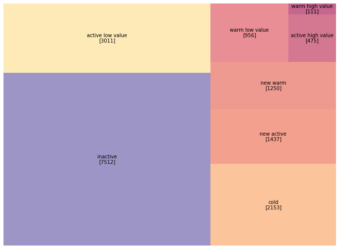
As we can see the figures have changed over the last year. Our new customers segment increased by more than 20% and inactive customers have drastically increased through the years so that half of our customer database is now inactive.
# The number of "new active high" customers has increased between 2014 and 2015.
# What is the rate of that increase?

ne = (customers_2015["segment"] == "active high value").sum()
ol = (customers_2014["segment"] == "active high value").sum()

print("New customers growth rate: %.0f%%" % round((ne - ol) / ol * 100))
New customers growth rate: 21%
Conducting a horizontal analysis such as the one addressed above is extremely valuable when it comes to gaining a more accurate and well-founded understanding of the evolution and challenges the company has been facing over the years. It enables managers to identify trends and growth patterns, determine the product lifecycle stage the product is currently in, as well as predict what the future may look like.
Building a Predictive Model
Forecasting involves building a statistical model by analyzing past and present data trends to predict future behaviors or to suggest actions to take for optimal outcomes. In this example, we decided to use a simple linear regression approach, using the customers’ RFM from 2014 as predictors and the revenue generated by those same customers in 2015 as target variables.
We first start by merging both dataframes: customers_2014 with revenue_2015 while making sure that new customers from 2015 are not included. We are going to call this new dataframe in_sample; meaning predictors and targets are already known.
# Merge 2014 customers and 2015 revenue
in_sample = customers_2014.merge(revenue_2015, how="left", on="customer_id")
# Transform NaN's to 0
in_sample["revenue_2015"].fillna(0, inplace=True)
Then we create a new variable active_2015, which indicates if a client made a purchase in 2015 or not and we set its type as int.
in_sample.loc[in_sample["revenue_2015"] > 0, "active_2015"] = 1
in_sample["active_2015"] = in_sample["active_2015"].astype("int")
in_sample.info()
<class 'pandas.core.frame.DataFrame'>
Int64Index: 16905 entries, 0 to 16904
Data columns (total 8 columns):
 #   Column          Non-Null Count  Dtype
---  ------          --------------  -----
 0   customer_id     16905 non-null  int64
 1   recency         16905 non-null  int64
 2   first_purchase  16905 non-null  int64
 3   frequency       16905 non-null  int64
 4   avg_amount      16905 non-null  float64
 5   max_amount      16905 non-null  float64
 6   revenue_2015    16905 non-null  float64
 7   active_2015     16905 non-null  int64
dtypes: float64(3), int64(5)
memory usage: 1.2 MB
The Likelihood a Customer will be Active in 2015
A powerful and relatively simple technique for calculating the probability of an event is logistic regression. In this section we are going to see how to use logistic regression to predict the likelihood a customer is going to be active in 2015. For that we are going to use statsmodels package, so make sure that you have it installed.
We start, of course, by importing statsmodels. This we have already done at the very top in the code section imports and it looks like this:
import statsmodels.api as sm
Then we define the model we want to apply using the R-Style formula string:
formula = "active_2015 ~ recency + first_purchase + frequency + avg_amount + max_amount"
prob_model = sm.Logit.from_formula(formula, in_sample)
This means that active_2015, which is our target variable, is a function of the following features: recency, first_purchase, frequency, avg_amount and max_amount; from the calibration dataframe in_sample.
Now we calibrate our model using the fit() method and extract the models coefficients as well as the standard deviations of those coefficients. In statsmodels, fit() returns an object containing the model coefficients, standard errors, p-values and other performance measures.
prob_model_fit = prob_model.fit()
# Extract the model coefficients
coef = prob_model_fit.params
# Extract their standard deviations
std = prob_model_fit.bse
Optimization terminated successfully.
         Current function value: 0.365836
         Iterations 8
From the results above, we can tell that the model successfully converges after completing only 8 iterations. Iterations refers to the number of times the model runs over the data in an attempt to optimize the model. The default is a maximum number of 35 iterations after which the optimization fails or doesn’t converge. The Current function value is the value of the loss function when we use the parameters found after calibration.
Just because our model converges is no guarantee that the results are accurate. The standard procedure for assessing whether the results of a regression can be trusted is to look at the so-called p-values. We can print them using the summary() method.
print(prob_model_fit.summary())
                           Logit Regression Results
==============================================================================
Dep. Variable:            active_2015   No. Observations:                16905
Model:                          Logit   Df Residuals:                    16899
Method:                           MLE   Df Model:                            5
Date:                Wed, 26 Oct 2021   Pseudo R-squ.:                  0.3214
Time:                        15:21:32   Log-Likelihood:                -6184.5
converged:                       True   LL-Null:                       -9113.9
Covariance Type:            nonrobust   LLR p-value:                     0.000
==================================================================================
                     coef    std err          z      P>|z|      [0.025      0.975]
----------------------------------------------------------------------------------
Intercept         -0.5331      0.044    -12.087      0.000      -0.620      -0.447
recency           -0.0020      6e-05    -32.748      0.000      -0.002      -0.002
first_purchase -1.167e-05   3.93e-05     -0.297      0.766   -8.86e-05    6.53e-05
frequency          0.2195      0.015     14.840      0.000       0.191       0.249
avg_amount         0.0004      0.000      1.144      0.253      -0.000       0.001
max_amount        -0.0002      0.000     -0.574      0.566      -0.001       0.000
==================================================================================
The p-value is listed above in the first table as LLR p-value. Typically, a p-value of 0.005 is considered statistically significant because there is only a 5% or less chance that these results are not valid. Along with the p-value for the entire regression, we can also find the p-values for each feature. They are listed in the above table under the variable P>|z|. From these values, we can see that the most important features of our regression model are recency and frequency.
From the standardized regression coefficients z, which are simply the regression coefficients divided by the standard errors, we can see that the recency parameter is quite large compared to the other parameters and is also negative. That is, the greater the recency or the more days that have elapsed between the last purchase and the current data, the less likely the customer is to make another purchase in the future. Which makes perfect sense.
# standardized regression coefficients z
print(coef/std)
Intercept        -12.09
recency          -32.75
first_purchase    -0.30
frequency         14.84
avg_amount         1.14
max_amount        -0.57
dtype: float64
So if your last purchase was two or three years ago, it is extremely unlikely that you will make a purchase in the near future. Indeed, the longer the period, the less likely you are to make a purchase. On the other hand, frequency is significantly large and positive. This means that the more purchases a customer has made in the past, the more likely s/he will make further purchases in the future. In fact, the ratio between coefficients and standard deviations indicates the extent to which a parameter is significant for our prediction model. As for the other features, they hardly play a role in the prediction, since they are all around zero.
Predicting the Dollar Value of the Next Purchase
Now that we have identified the customers who are more likely to make a purchase in 2015, let’s put a dollar value on their upcoming transaction. The problem here is that our model can only be calibrated on those customers who actually bought something in 2015. Hence, we have to resample our in_sample dataset so that only customers who were active in 2015 are taken into account. Actually, only their customers ID would do.
# For the monetary model, we select only those who made a purchase
# Only  index  suffice, since it represents the customer's ID
z = in_sample[in_sample["active_2015"] == 1].index.tolist()

# Let's print the 5 first customers ID's
z[:5]
[1, 17, 29, 30, 31]
It looks good. Let’s now print some descriptive statistics using describe().
       customer_id  recency  first_purchase  frequency  avg_amount  \
count     3,886.00 3,886.00        3,886.00   3,886.00    3,886.00
mean    134,906.97   306.35        1,636.16       4.74       67.78
std      68,404.30   519.46        1,101.25       3.79      160.06
min          80.00     1.00            1.00       1.00        5.00
25%      78,590.00    23.00          649.75       2.00       30.00
50%     143,550.00    97.00        1,604.00       4.00       40.00
75%     194,362.50   328.00        2,666.00       7.00       60.00
max     236,660.00 3,544.00        3,647.00      40.00    4,500.00

       max_amount  revenue_2015  active_2015
count    3,886.00      3,886.00     3,886.00
mean        88.33         92.30         1.00
std        222.15        217.45         0.00
min          5.00          5.00         1.00
25%         30.00         30.00         1.00
50%         50.00         50.00         1.00
75%         80.00        100.00         1.00
max      4,500.00      4,500.00         1.00
As expected, we only have customers that were active in 2015.
In terms of sales, customers spent between $5 and $4,500 in our store in 2015. Let’s now calibrate our monetary model. We start by estimating 2015 spending based on two attributes: the average amount they typically spend and the maximum amount spent. These are the predictors. Since this is not a classification problem but rather a linear prediction problem with continuous target variables, logistic regression would be inappropriate in this case.
OLS, short for ordinary least squares, is probably the most commonly used regression model for this type of task. It attempts to find the line of best fit for the given data by minimizing the sum of squared residuals between the prediction line and the actual data.
# Calibrate the monetary model (version 1)
amount_model = sm.OLS.from_formula(
    "revenue_2015 ~ avg_amount + max_amount", in_sample.loc[z]
)
amount_model_fit = amount_model.fit()
Let’s print a summary of our OLS regression model.
print(amount_model_fit.summary())
                            OLS Regression Results
==============================================================================
Dep. Variable:           revenue_2015   R-squared:                       0.605
Model:                            OLS   Adj. R-squared:                  0.605
Method:                 Least Squares   F-statistic:                     2979.
Date:                Thu, 27 Oct 2021   Prob (F-statistic):               0.00
Time:                        21:10:39   Log-Likelihood:                -24621.
No. Observations:                3886   AIC:                         4.925e+04
Df Residuals:                    3883   BIC:                         4.927e+04
Df Model:                           2
Covariance Type:            nonrobust
==============================================================================
                 coef    std err          t      P>|t|      [0.025      0.975]
------------------------------------------------------------------------------
Intercept     20.7471      2.381      8.713      0.000      16.079      25.415
avg_amount     0.6749      0.033     20.575      0.000       0.611       0.739
max_amount     0.2923      0.024     12.367      0.000       0.246       0.339
==============================================================================
Omnibus:                     5580.836   Durbin-Watson:                   2.007
Prob(Omnibus):                  0.000   Jarque-Bera (JB):          8162692.709
Skew:                           7.843   Prob(JB):                         0.00
Kurtosis:                     226.980   Cond. No.                         315.
==============================================================================

Notes:
[1] Standard Errors assume that the covariance matrix of the errors is correctly specified.
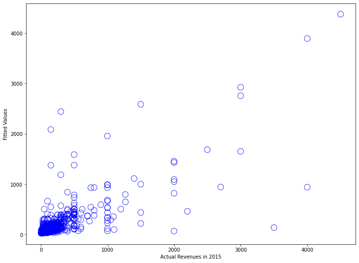
As we can see from the statistical summary, both selected features are statistically significant. Furthermore, the R-squared value is 0.61, which means that 61% of the variation in the output variables is explained by the input variables. This is not bad at all. In fact, an R-squared value of more than 0.6 indicates a fitting model. And at 60.5%, we are slightly above that figure. That said, let’s plot the results to see how good or bad our predictions are.
plt.scatter(in_sample.loc[z].revenue_2015, amount_model_fit.fittedvalues);
Statsmodels provides a number of convenient plot functions to illustrate the regression models in more details. For instance, we use the function plot_regress_exog to quickly check the model assumptions with respect to a single regressor, in our case avg_amount.
sm.graphics.plot_regress_exog(amount_model_fit, 'avg_amount');
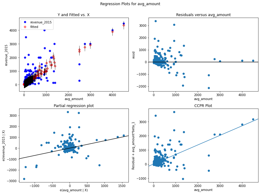
That doesn’t look good, and the reason is that most of the customers spent quite small amounts. Mostly between 50 and 200 dollars. Only a few outliers have spent large amounts, up to four thousand dollars. However, the model tries to draw a line through this cloud of points where no line would really make sense.
When dealing with skewed data, it is recommended to perform a logarithmic transformation. This is indeed a convenient method and by far the most commonly used technique for normalizing highly skewed data. So instead of predicting 2015 revenue based on the average amount and the maximum amount. We will predict the logarithm of 2015 revenues based on the logarithm of the average and the maximum amount. So let’s see how it works.
# Re-calibrate the monetary model, using a log-transform (version 2)
amount_model_log = sm.OLS.from_formula(
    "np.log(revenue_2015) ~ np.log(avg_amount) + np.log(max_amount)", in_sample.loc[z]
)
amount_model_log_fit = amount_model_log.fit()
print(amount_model_log_fit.summary())
                             OLS Regression Results
================================================================================
Dep. Variable:     np.log(revenue_2015)   R-squared:                       0.693
Model:                              OLS   Adj. R-squared:                  0.693
Method:                   Least Squares   F-statistic:                     4377.
Date:                  Fri, 28 Oct 2022   Prob (F-statistic):               0.00
Time:                          00:31:16   Log-Likelihood:                -2644.6
No. Observations:                  3886   AIC:                             5295.
Df Residuals:                      3883   BIC:                             5314.
Df Model:                             2
Covariance Type:              nonrobust
======================================================================================
                         coef    std err          t      P>|t|      [0.025      0.975]
--------------------------------------------------------------------------------------
Intercept              0.3700      0.040      9.242      0.000       0.292       0.448
np.log(avg_amount)     0.5488      0.042     13.171      0.000       0.467       0.631
np.log(max_amount)     0.3881      0.038     10.224      0.000       0.314       0.463
==============================================================================
Omnibus:                      501.505   Durbin-Watson:                   1.961
Prob(Omnibus):                  0.000   Jarque-Bera (JB):             3328.833
Skew:                           0.421   Prob(JB):                         0.00
Kurtosis:                       7.455   Cond. No.                         42.2
==============================================================================

Notes:
[1] Standard Errors assume that the covariance matrix of the errors is correctly specified.
We can already see that our model slightly improved. In fact, the R-squared score got better and the intercept std err is now much lower, meaning that we fit the data much better.
# Plot the results of the monetary model
# Plot the results of the monetary model
plt.scatter(np.log(in_sample.loc[z].revenue_2015), amount_model_log_fit.fittedvalues,
           alpha=.8, facecolors='none', s=140, edgecolors='b')
plt.xlabel('Log of the Revenues in 2015')
plt.ylabel('Log Fitted Values');
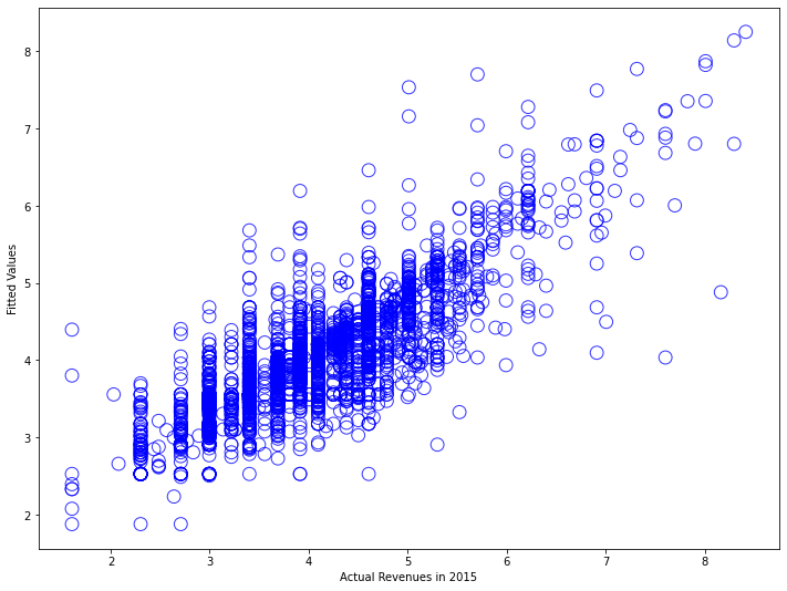
This looks much better than before. We can now imagine a nice line tracing through this point cloud and more accurately predicting 2015 revenue based on the new model we just created. By performing the logarithmic transformation, we weighted the smaller values more and the very large values less, resulting in a quasi-normalized distribution of our data.
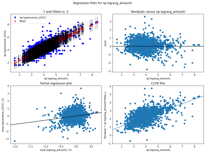
sm.graphics.plot_regress_exog(amount_model_log_fit, 'np.log(avg_amount)');
Applying the Models to Today’s Data
So let’s briefly summarize what we’ve done so far. We have calibrated two models, the first to predict the probability that a customer will be active. For that we used logistic regression. The second; a linear OLS regression model on log transformed data, to predict how much they will spend if they were active in 2015. Now the objective of this section is to use both models to forecast future transactions. So bear with me for a little while.
So we want to look at the behavior of our customers today. For that, we start by extracting exactly the same information that we used to forecast a year ago. That is frequency, recency, first purchase, average amount and maximum amount for all customers from 2015. We’ve already done that somewhere above.
# Compute RFM as of Today
q = """
        SELECT customer_id,
        MIN(days_since) AS 'recency',
        MAX(days_since) AS 'first_purchase',
        COUNT(*) AS 'frequency',
        AVG(purchase_amount) AS 'avg_amount',
        MAX(purchase_amount) AS 'max_amount' FROM df GROUP BY 1
"""
customers_2015 = sqldf(q, globals())
Unlike the previous section, now we do not know who will be active next year and how much they will spend. As a reminder, today is January 1st, 2016 and the task is to predict the activity of customers during this year. For this we are going to apply the two models that we have generated above to our actual data; namely customers_2015. Let’s see how this works.
We start by predicting the probability that a customer is going to be active during 2016. For that we use the first generated regression model prob_model_fit. The prediction is done using the predict() method from statsmodels and the results are saved under prob_predicted.
# Predict the target variables based on today's data
# 1st: we predict the probability that a customer is going to be in 2016 active
customers_2015["prob_predicted"] = prob_model_fit.predict(customers_2015)

# Results summary
customers_2015.prob_predicted.describe()
count   18,417.00
mean         0.22
std          0.25
min          0.00
25%          0.01
50%          0.11
75%          0.40
max          1.00
Name: prob_predicted, dtype: float64
From above we can see that customers have on average a 22% probability of being active. For some customers, it is absolutely certain that they will be active; these have a probability of almost one. For others, it is absolutely certain that they will not be active; for these, the probability is close to zero. Most customers lie in between.
Now, we want to use the second regression model to predict the dollar value of customer activity. Recall that we had to use a logarithmic transformation to get around the skewness of the input data. This means we want to take the exponential values of the model output. The results are then saved as a new variable revenue_predicted in our dataframe customers_2015.
# 2nd we predict the revenue
# Since our model predicts the log(amount) we need to take the exponential of
# the predicted revenue generated per customer
customers_2015["revenue_predicted"] = np.exp(amount_model_log_fit.predict(customers_2015))

# Print results summary
customers_2015.revenue_predicted.describe()
count   18,417.00
mean        65.63
std        147.89
min          6.54
25%         29.00
50%         35.05
75%         57.30
max      3,832.95
Name: revenue_predicted, dtype: float64
Looking at the expected sales of active customers, that is, how much they will spend on average in the coming year, this figure is about $65, while the range here is between $6 and $3,800. And, of course, the minimum value is $6, not zero, because the second regression model assumes that all customers will be active. Therefore, it is necessary to determine the probability that a customer is active and include it in the prediction so that we get an overall measure of the customer’s spending in the next year.
Thus, the final stage of the prediction consists of assigning each customer a score indicating how likely they are to take action in conjunction with how much money they will spend.
# 3rd: we give a score to each customer which is the conjunction of probability
# predicted multiplied by the amount.
customers_2015["score_predicted"] = (
    customers_2015["prob_predicted"] * customers_2015["revenue_predicted"]
)

# Print results summary
customers_2015.score_predicted.describe()
count   18,417.00
mean        18.83
std         70.21
min          0.00
25%          0.46
50%          4.56
75%         17.96
max      2,854.16
Name: score_predicted, dtype: float64
So the total score is a function of both probability and revenue combined. And the score has a mean value of 18.8. From a managerial perspective, this value is extremely important. It means that each customer in this database will spend an average of $18.8 in the upcoming year. Many will spend nothing, some may spend $333, others $50, but on average it will probably be $18.8.
From a marketing perspective, it is better to focus our activities on customers with high scores, as this means they are likely to be the most profitable for the company.
Assuming we want to reach only the customers with a score higher than $50, this can be done as follows:
# How many customers have an expected revenue of more than $50
z = customers_2015[customers_2015.score_predicted > 50].index.tolist()
print(len(z))
1324
The above code fragment creates a vector of customers that have a score above 50 ($). There are 1,323 customers in total. So out of the list of 18,000 customers, only about 1,300 have a predicted to spend more than $50 throughout 2016. These should be your target customers. You can determine their ID or number by simply adding the following line to your code:
# Customers with the highest score:
customers_2015["customer_id"].loc[z]
1            80
17          480
29          830
30          850
31          860
          ...
16892    234210
16895    234240
16896    234250
16897    234260
16903    234320
Name: customer_id, Length: 3886, dtype: int64
As output we obtain a list of the customer numbers of all those who are expected to spent more that 50$ in our shop. Now only you now whom to target and how.
Conclusion
In this tutorial, we have demonstrated how to predict customers’ next year’s purchases and the amount of dollars they will spend at your store. Our predictions are based on RFM analysis combined with linear regressions. We used two different linear regression approaches: Logistic Regression and Ordinary Least Squares (OLS) to generate a score for each customer.
With logistic regression, we were able to predict the probability of customer activity in the next financial period. It is a classification algorithm with two outputs; 0 or 1. The results are weighted and the weights are nothing more than the probability that the customer will be active. That is, the larger the weighting, the more likely it is a customer may be active in a given period.
Then we used OLS to predict the dollar value of the customers’ purchases over the same financial period. Finally, we built the score by linking the two results together. The scores are in Dollar and reflect the customers next years revenues. They can be used as the basis for many strategic decisions, as well as new segmentation guidelines.
I hope that by now you are convinced of the importance and versatility of RFM analysis, especially when combined with statistical learning. In case you still have doubts or are not sure about integrating it into your business analysis, read my next tutorial.
References
- Lilien, Gary L, Arvind Rangaswamy, and Arnaud De Bruyn. 2017. Principles of Marketing Engineering and Analytics. State College, PA: Decisionpro.
- Arnaud De Bruyn. Foundations of marketing analytics (MOOC). Coursera.
- Dataset from Github repo. Accessed 15 December 2021.
Business Analytics Tutorial RFM Analysis Customer Segmentation 