Forecasting Customer Lifetime Value Using RFM-Analysis and Markov Chain
Introduction
If there’s one thing you should be doing in your business right now, and I’m willing to bet you’re not, it’s Customer lifetime value (CLV) analysis.
CLV is the present value of the future cash flows or payments a company will realize from a customer over the entire relationship. It helps businesses understand how to best use their marketing budget and strategies to grow their customer base. For instance, by understanding CLV, a business can determine how much it can afford to spend to acquire a new customer, identify and target future top customers or minimize spending for unprofitable customers.
In fact, whenever a business makes a decision about a customer relationship, it wants to make sure that the decision is going to be profitable in the long run.
In this article, we will demonstrate how to use Python to implement a CLV forecasting model. It’s important to note that we assume a non-contractual business setting. In a contract-based business, customers are typically locked into long-term agreements, where they pay the same fee on a recurring basis,making it relatively easy to estimate CLV based on retention rate.
However, in a non-contractual environment, where customers can come and go as they please, estimating variable future revenue streams in terms of time and amount can be more challenging.
Fortunately, we’ve already addressed similar issues in previous articles and know that nothing beats the RFM trinity when it comes to predicting customer behavior. So, if you are unfamiliar with RFM-analysis (recency, frequency, monetary value), take a moment to read my previous article.
Now, before I get into the code, I’d like to briefly discuss some of the theory. Those who are simply interested in programming can skip the next three sections and go straight to CLV in Python.
From Product-Centric to Customer-Centric Marketing
Until recently, retailers have approached marketing from a product-oriented perspective, focusing mainly on the features, benefits, and prices of their products and services while ignoring the needs and wants of their customer base. The focus of this approach is on quick transactions, using marketing mix and advertising campaigns to grab new consumers’ attention and persuade them to make an impulse purchase. Sales are then treated as faceless transactions with the ultimate goal to increase conversion and short-term profits.
However, in today’s competitive business landscape, retailers are looking for new ways to differentiate themselves from their competitors. Those that adopt customer-centric marketing can provide tailored experiences that are engaging for their customer base. This requires understanding customers on an individual level and forecasting their CLV to determine how profitable they will be in a long-term relationship. After all, you don’t want to waste your time and marketing budget on unprofitable customers.
Indeed, the transition to a more customer-centric marketing strategy among retailers comes from a combination of factors such as competitive pressures, changing consumer behavior, digital transformation and data availability.
With the advent of social media and e-commerce, customers have gained greater access to a variety of retailers offering the same or similar products and have become more knowledgeable in their purchasing decisions. They now expect organizations to understand and cater to their individual needs and wants, and have higher expectations for personalized and tailored value-added services and buying experiences.
In addition, digital transformation and the availability of data have made it easier for retailers to gain insights into customers’ behavior, preferences and concerns. This data can be used to create more targeted and personalized marketing campaigns and improve products and services. Customer relationship management (CRM) tools also enabled retailers to manage customer interactions more efficiently and effectively while improving overall customer satisfaction and retention.
In summary, it is essential for organizations to adopt both product and customer-centric marketing strategies to remain competitive in saturated marketplaces.
A customer-centric approach is important for building strong relationships with the customer base and fostering trust and loyalty, which can attract repeat purchases, increase word of mouth and prevent customers from turning to competitors. On the other hand, a product-centric approach is also important when it comes to attracting new customers and generating initial interest in a product or service.
By using both strategies, retailers can effectively balance the needs of new customer acquisition and customer retention, ultimately leading to long-term success in the marketplace.
Motivation and Use Cases
Imagine your company launches a big campaign to attract new customers. You invest in PR, advertising and email campaigns, buy a lot of online ads, create a special promotion and offer a big discount to first-time buyers. However, after all these efforts, the campaign results in only a small number of new customers and sales that don’t even cover the cost of the campaign. Well, you could argue that these new customers will stay with you and continue to buy, making the campaign worthwhile in the long run. But wouldn’t it be nice to have a way to measure whether or not that’s true? That’s where customer lifetime value (CLV) models come in. These models look at past and current customer behavior to predict how much revenue a customer will bring in over time. Only then can you determine if the cost of customer acquisition was worth it.
CLV models offer a wide range of practical applications. For example, you might compare one acquisition campaign to another. Suppose you are comparing two campaigns, one with a substantial discount and one with a modest discount. The advertising campaign with the greater discount will likely attract more customers, but those customers will be less profitable in the short term and much less loyal in the long term once the discount is removed. After all, the only reason they came in the first place was to take advantage of the discount. Offering a small discount and bringing in fewer customers might be a better strategy, assuming of course, they are more loyal and bring in more money in the long run. But how can you be sure about that, if you can’t quantify the long-term value of your customers.
CLV is also very useful for existing customers. In fact, one of the best uses of Customer Lifetime Value is to determine which customers or customer segments are more valuable to the future growth of your business. Let’s say you have two segments, with customers in segment one contributing an average of $100 per quarter to revenue. Customers in segment two generate an average of $150. At first glance, you might want to put a little more effort into satisfying and retaining the customers in segment two. Perhaps additional resources should be allocated. Make sure they have access to the best customer service possible. Keep an eye on loyalty, and so on. However, an analysis of their lifetime value shows that customers in the first segment are more loyal, stay longer, and regularly spend more money with the company. Customers in the second segment are simply seasonal and not loyal at all. They switch to the competition as soon as they discover a better offer or special promotion, and may only be one-time customers. Comparing lifetime values, customers in the first segment spend an average $5,000 during all they relationship with your company, while customers in segment two spend an average of only $600. Wouldn’t it be wonderful if you knew how to calculate these numbers in the first place so you could focus your marketing resources on the most valuable customers over time? What do you think would happen if you didn’t?
The Migration Model
CLV can be tricky to compute. Some methods are too simplistic to be useful, while others are too complex. In this tutorial, we’ll take a middle-of-the-road approach and use segmentation - a concept we’ve already covered in previous articles - to compute CLV.
You may recall that we talked about managerial segmentation, where you can assign customers to different segments based on their behaviors like recency, frequency, monetary value (RFM). We also discussed how you can use this segmentation not just on current data, but also retrospectively on past data. This provides significant information into how your business is performing, which segments are increasing and on the account of what other segments, and whether you’re attracting more new consumers than before.
Each segmentation is like a snapshot of your customer database. By taking multiple snapshots over time, you can see how customers move from one segment to another. For example, some high-value customers may stay in the same segment while others move to lower-value segments. By analyzing these transitions, you can predict how your customers will behave in the future.
To make this easier, we will use a tool called a transition matrix, also known as migration model. It is a mathematical representation of the transition probabilities of a Markov chain. It is a square matrix and in this case shows the probability of customers moving from one segment to another. Each row represents the current segment, while each column represents the segment customers were in a year ago. The sum of each row should equal 1, which means that the probabilities of switching from one state to another are equal to 1. It’s important to note that by definition, some transitions may have zero probability, such as a customer moving from active to inactive in just one period. This is normal and expected.
Based on the analysis of this matrix, you can predict how customers will behave in the future.
Forecasting Customer Lifetime Value in Python
Now that we are done with the theory, let’s move on to the implementation. In the following we want to implement a CLV model using RFM and a first-order Markov chain. We will reuse the same data as in the previous blog post, as well as the first part of implementation, which includes RFM analysis and customer segmentation for the year 2014. The data consists of 51,243 observations across three variables:
- Customer ID,
- purchase amount in USD and
- date of purchase
It includes all sales from January 2, 2005 through December 31, 2015. There are no missing records in the dataset.
RFM Analysis and Customer Segmentation for The Current Year
I assume by now you are familiar with the dataset and customer segmentation techniques, so I won’t go into detail here. I’m going to load the dataset, set it up as we’ve done before, and then I’m going to segment it based on RFM analysis, with the assumption that we’re at the end of 2015.
# import needed packages
import matplotlib as mpl
import matplotlib.pyplot as plt
import numpy as np
import pandas as pd
import patsy
import squarify
import statsmodels.api as sm
from pandasql import sqldf
from tabulate import tabulate

# Set up the notebook environment
pysqldf = lambda q: sqldf(q, globals())
%precision %.2f
pd.options.display.float_format = "{:,.2f}".format
plt.rcParams["figure.figsize"] = 10, 8

# Load text file into a local variable
columns = ["customer_id", "purchase_amount", "date_of_purchase"]
df = pd.read_csv("purchases.txt", header=None, sep="\t", names=columns)

# interpret the last column as datetime
df["date_of_purchase"] = pd.to_datetime(df["date_of_purchase"], format="%Y-%m-%d")

# Extract year of purchase and save it as a column
df["year_of_purchase"] = df["date_of_purchase"].dt.year

# Add a day_since column showing the difference between last purchase and a basedate
basedate = pd.Timestamp("2016-01-01")
df["days_since"] = (basedate - df["date_of_purchase"]).dt.days

# SQL for the RFM analysis
q = """
        SELECT customer_id,
        MIN(days_since) AS 'recency',
        MAX(days_since) AS 'first_purchase',
        COUNT(*) AS 'frequency',
        AVG(purchase_amount) AS 'amount'
        FROM df GROUP BY 1"""
customers_2015 = sqldf(q)

# Customer segmentation in 2015
customers_2015.loc[customers_2015['recency'] > 365*3, 'segment'] = 'inactive'
customers_2015['segment'] =  customers_2015['segment'].fillna('NA')
customers_2015.loc[(customers_2015['recency']<= 365*3) &
                   (customers_2015['recency'] > 356*2), 'segment'] = "cold"
customers_2015.loc[(customers_2015['recency']<= 365*2) &
                   (customers_2015['recency'] > 365*1), 'segment'] = "warm"
customers_2015.loc[customers_2015['recency']<= 365, 'segment'] = "active"
customers_2015.loc[(customers_2015['segment'] == "warm") &
                  (customers_2015['first_purchase'] <= 365*2), 'segment'] = "new warm"
customers_2015.loc[(customers_2015['segment'] == "warm") &
                  (customers_2015['amount'] < 100), 'segment'] = "warm low value"
customers_2015.loc[(customers_2015['segment'] == "warm") &
                  (customers_2015['amount'] >= 100), 'segment'] = "warm high value"
customers_2015.loc[(customers_2015['segment'] == "active") &
                  (customers_2015['first_purchase'] <= 365), 'segment'] = "new active"
customers_2015.loc[(customers_2015['segment'] == "active") &
                  (customers_2015['amount'] < 100), 'segment'] = "active low value"
customers_2015.loc[(customers_2015['segment'] == "active") &
                  (customers_2015['amount'] >= 100), 'segment'] = "active high value"

# Transform segment column datatype from object to category
customers_2015["segment"] = customers_2015["segment"].astype("category")
# Re-order segments in a better readable way
sorter = [
    "inactive",
    "cold",
    "warm high value",
    "warm low value",
    "new warm",
    "active high value",
    "active low value",
    "new active",
]
customers_2015.segment.cat.set_categories(sorter, inplace=True)
customers_2015.sort_values(["segment"], inplace=True)
You can do 2014 by yourself. It is almost the same as with 2015. The only minor difference resides in the SQL query. Hint: Remember we are in 2014, so we want to filter out everything after 2014 and don’t forget to order the segments exactly as for 2015.
Transition Matrix
Well, now we have all the information we need. We have the customers and their segments for both 2014 and 2015. Next, we need to merge these two datasets into one new variable. However, there is a trick to this. The columns in each dataset have the same names, so if we merge them simply, they will overwrite each other. To avoid this, we will specify that we want to merge them by customer ID and keep all the customers from the left dataset as we’ve done before.
# merge both customer segmentation years
new_data = customers_2014.merge(customers_2015, how='left', on='customer_id')

new_data.info()
<class 'pandas.core.frame.DataFrame'>
Int64Index: 16905 entries, 0 to 16904
Data columns (total 11 columns):
 #   Column            Non-Null Count  Dtype
---  ------            --------------  -----
 0   customer_id       16905 non-null  int64
 1   recency_x         16905 non-null  int64
 2   first_purchase_x  16905 non-null  int64
 3   frequency_x       16905 non-null  int64
 4   amount_x          16905 non-null  float64
 5   segment_x         16905 non-null  category
 6   recency_y         16905 non-null  int64
 7   first_purchase_y  16905 non-null  int64
 8   frequency_y       16905 non-null  int64
 9   amount_y          16905 non-null  float64
 10  segment_y         16905 non-null  category
dtypes: category(2), float64(2), int64(7)
memory usage: 1.3 MB
Now, we have a large dataset with columns for recency, first purchase, frequency, amount, and segments with an _x or _y appended to the column name. The _x columns represent the data from the 2014 customers and the _y columns represent the data from the 2015 customers.
The two columns that we’re interested in are segment_x and segment_y, which represent the segments for the customers in 2014 and 2015, respectively.
# Let's print the obtained segment_x and segment_y columns
print(tabulate(new_data[['customer_id', 'segment_x', 'segment_y'
                         ]].tail(), headers='keys', tablefmt='psql')
      )
+-------+---------------+-------------+------------------+
|       |   customer_id | segment_x   | segment_y        |
|-------+---------------+-------------+------------------|
| 16900 |        221470 | new active  | new warm         |
| 16901 |        221460 | new active  | active low value |
| 16902 |        221450 | new active  | new warm         |
| 16903 |        221430 | new active  | new warm         |
| 16904 |        245840 | new active  | new warm         |
+-------+---------------+-------------+------------------+
To further analyze the data, I’m going to create a cross-tabulation (or “occurrence table”) that shows how many customers fit into specific segment combinations for both 2014 and 2015. This will allow us to see how many customers moved between segments or stayed in the same segment between the two years.
# We are going to cross segments 2014 and 2015 and see how many people are
# in both an meet this criterium
transition = pd.crosstab(new_data['segment_x'], new_data['segment_y'])
print(transition)
segment_y          inactive  cold  warm high value  warm low value  new warm  \
segment_x
inactive               7227     0                0               0         0
cold                   1931     0                0               0         0
warm high value           0    75                0               0         0
warm low value            0   689                0               0         0
new warm                  0  1139                0               0         0
active high value         0     0              119               0         0
active low value          0     0                0             901         0
new active                0     0                0               0       938

segment_y          active high value  active low value
segment_x
inactive                          35               250
cold                              22               200
warm high value                   35                 1
warm low value                     1               266
new warm                          15                96
active high value                354                 2
active low value                  22              2088
new active                        89               410
If we examine the results, we can see that we are almost there. The table above closely resembles the transition matrix we discussed earlier. The rows represent the segments that customers belonged to in 2014: segment_x. The columns show the different segments that customers moved to in 2015 or segment_y. Each value in the table represents the number of customers who moved from one segment to another between the two years.
For example, among all the inactive customers in 2014, 7,227 remained inactive in 2015, 35 became active high value customers, and 250 became active low value customers. Additionally, among all the new active customers in 2014, 938 didn’t purchase anything the next year and became new warm customers. That’s about two out of three new customers. The others became active high value or active low value customers.
However, we don’t really care about the absolute numbers, what we care about are the proportions, likelihoods, and probabilities of shifting from one segment to the next over time. So instead of working with the absolute numbers as represented in the above table, we will divide each row by the row sum. This will give us a table where the sum of each row is equal to one.
transition = transition.apply(lambda x: x/x.sum(), axis=1)
print(transition)
segment_y          inactive  cold  warm high value  warm low value  new warm  \
segment_x
inactive               0.96  0.00             0.00            0.00      0.00
cold                   0.90  0.00             0.00            0.00      0.00
warm high value        0.00  0.68             0.00            0.00      0.00
warm low value         0.00  0.72             0.00            0.00      0.00
new warm               0.00  0.91             0.00            0.00      0.00
active high value      0.00  0.00             0.25            0.00      0.00
active low value       0.00  0.00             0.00            0.30      0.00
new active             0.00  0.00             0.00            0.00      0.65

segment_y          active high value  active low value
segment_x
inactive                        0.00              0.03
cold                            0.01              0.09
warm high value                 0.32              0.01
warm low value                  0.00              0.28
new warm                        0.01              0.08
active high value               0.75              0.00
active low value                0.01              0.69
new active                      0.06              0.29
Well that looks better. So, if you were an inactive customer in 2014, you had a 96.2% chance of remaining inactive in 2015. And if you were an active high value customer, you had a 74.5% chance of remaining in that segment and a 25% chance of becoming a warm high value customer next year.
That’s actually all we need for now. The next step is to use this transition matrix to make predictions.
Using Transition Matrix to Make Predictions
In the previous section we showed how to create a transition matrix. Once we have it, the next step is to estimate the number of customers we will have in each segment in the future. This can be done for any number of years, although most companies will stop after three, five, or at most ten years.
To estimate these numbers, we need to consider two things: the transition matrix and the current number of customers in each segment. Remember, the transition matrix shows how customers got to where they are today. We will use the same information to estimate where they will be in the future.
Without going into too much mathematical detail, this process involves multiplying a matrix by a vector. To do this, we multiply the transition matrix by a vector representing the number of customers in each segment to date. The result of this process is then a new vector containing the estimated number of customers in each segment next year. By multiplying this new vector again by the same transition matrix, we can estimate the number of customers in each segment two years from now, and so on.
We will now look at how this can be achieved in Python:
So, we have a transition matrix that shows the likelihood of customers moving from one segment to another over one year. To use this information, we will prepare a matrix or placeholder to store our predictions. The number of rows in this matrix will be the number of segments we have, and the number of columns will be the number of years we are predicting the evolution of segment membership. In this case, we are going to predict over ten periods in the future and include one more for the present. So, we start by creating an empty 8x11 matrix.
The first thing we need to do is to populate the first column with the number of customers in each segment as of the end of 2015. And then, we’ll give each row the name of its corresponding segment.
# Initialize a placeholder matrix with then number of customers in each segment today
# and after 10 periods.
# The number of rows is the number of segments we have
# The number of columns is the number of years we are going to predict -
# The evolution of segment membership
segments = np.zeros(shape=(8,11))

# 1st thing to do is to populate the first columns with then number of
# customers in each segment at the end of 2015
segments[:, 0] = customers_2015['segment'].value_counts(sort=False)

# 2nd Give each column the name of its corresponding year
# and row the name of its corresponding segment:
segments = pd.DataFrame(segments, columns=np.arange(2015,2026), index=customers_2015['segment'].values.categories)
As a result, we should see only the 2015 column filled with positive numbers, and all other years showing 0’s. Now, we would like to fill out these columns with predictions made using the transition matrix. So, for each column, the segments over that year would be a function of segments of the year before, multiplied by the transition matrix. To do that, we use a loop over all the given years, where each generated column is multiplied with the transition matrix and added to the next column, until we reach the end of the loop, which will be the year 2025.
# Compute for each an every period
for i in range(2016, 2026):
    segments[i] = segments[i-1].dot(transition).round(0)
    segments[i].fillna(0, inplace=True)

# Noneed for float64 since we are rounding the results:
segments = segments.astype(int)
Now, if you look at the matrix we just created, it contains the segment names, the years, and the number of customers (rounded) in each segment at that time. We rounded the numbers because it doesn’t make sense to predict that we’ll have 0.4 customer in a segment.
# print resulting matrix
print(segments, headers='keys', tablefmt='psql')
                   2015   2016   2017   2018   2019   2020   2021   2022  \
inactive           9158  10517  11539  12636  12940  13185  13386  13542
cold               1903   1584   1711    874    821    782    740    709
warm high value     119    144    165    160    157    152    149    146
warm low value      901    991   1058    989    938    884    844    813
new warm            938    987      0      0      0      0      0      0
active high value   573    657    639    625    608    594    582    571
active low value   3313   3537   3306   3134   2954   2820   2717   2637
new active         1512      0      0      0      0      0      0      0

                    2023   2024   2025
inactive           13664  13760  13834
cold                 685    665    651
warm high value      143    141    139
warm low value       789    771    756
new warm               0      0      0
active high value    562    554    548
active low value    2575   2527   2490
new active             0      0      0
Let’s now plot the evolution of inactive customers over all the forecasted years as a bar plot.
# Plot inactive customers over time
segments.iloc[0].plot(kind='bar')
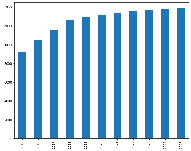
These are our predictions. We begin at around 9,158, and then we expect the number of inactive customers to grow quickly and then stabilize around 13,000. You can do that in other segments and see how they change overtime.
If you take a look at the last row in the table above, specifically the number of new active customers, you’ll notice that we have 1,512 in 2015 and zeros in all other years. This is because once a customer is already in the database, they cannot become new again. The only way for a customer to become new is to be acquired. In this case, we are only measuring the CLV of those customers who are already in the database. This means that new active customers will eventually become something else, like warm, active, cold, or inactive customers over time. Thus, this segment will remain empty unless we run acquisition campaigns and add new customers to the database.
Now, we don’t have any forecast of the generated revenues yet, and that’s what we’re going to do in the next section.
Computing CLV
Now that we have the number of customers per segment for each year, we just need to convert these figures into dollars or euros. The first step is to assume that the revenue generated by a customer can be fully explained and predicted by the segment to which they belong, whether it’s today or ten years from now.
For instance, if customers in high-value segment generates on average $600, we’ll assume that this figure will not change over the years. In reality, it might go up or down, but without additional information, our best guess is to assume that this figure will remain stable over time. However, we need to take into account the time value of money when calculating CLV, as a dollar received today is worth more than a dollar received in the future. This is where discounting comes in. By discounting future revenues, we can compare them to today’s acquisition costs and determine if it’s a good investment. So discounting is a way of adjusting the value of money received or paid in the future to its present value. This means that the longer you have to wait to generate revenues from a customer segment, the less valuable they will be for your organization today.
So let’s translate that into a Python code. We start first by computing the average revenue per customer per segment. That we’ve already done in the previous blog entry and looks as follows:
# Show average revenue per customer and per segment
aggregate(x = actual$revenue_2015, by = list(customers_2015$segment), mean)
Customers who were inactive, cold, warm, by definition generate no revenue at all. The active high value customers on average generate $323 of revenue per year. And then for the active low value and new active, it goes down to $52 and $79. So we’re going to just take the data from that analysis and store it, in a variable called average_revenue.
# Average yearly revenue per segment
# This comes directly from the previous post
average_revenue = [0, 0, 0, 0, 0, 323.57, 52.31, 79.17]
Now we take the variable called segments, which contains predictions of segment membership over the next 11 years and multiply it by how much revenue each segment generated in average by 2015. As result we get an 8x11 matrix showing a forecast of how much each segment will generate over the next 10 years.
# Compute revenue per segment
revenue_per_segment = segments.multiply(average_revenue, axis='index')
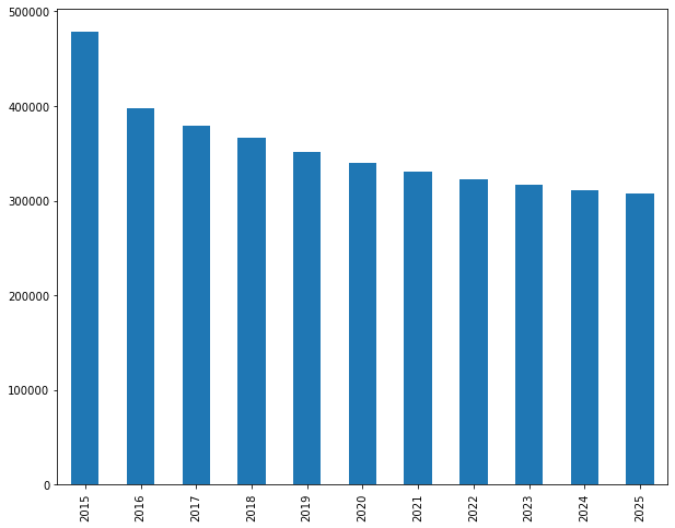
The next step to do is to compute the sum of each column, that is yearly revenues, and we store the result under yearly_revenue.
# Compute yearly revenue
yearly_revenue = revenue_per_segment.sum(axis=0).round(0)
yearly_revenue
2015   478,414.00
2016   397,606.00
2017   379,698.00
2018   366,171.00
2019   351,254.00
2020   339,715.00
2021   330,444.00
2022   322,700.00
2023   316,545.00
2024   311,445.00
2025   307,568.00
dtype: float64
We can see that we’ve generated $478,000 in 2015. However, over time as customers become inactive, this number will decrease, and by 2025 we’ll have without discounting only $307,000 in revenue. We can also create a bar plot to visualize this decrease in revenue over time.
yearly_revenue.plot(kind='bar')
If we want to calculate the cumulative revenue over the years, also known as Customer Equity (CE) we can use the cumsum function on the yearly_revenue variable.
# Compute cumulated revenue
cumulated_revenue = yearly_revenue.cumsum(axis=0)
print(cumulated_revenue.round(0))
cumulated_revenue.plot(kind='bar')
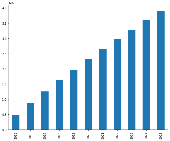
As you can see, the cumulative revenue can only increase as we add new revenue each year. However, the slope of the curve will slowly decrease as we lose revenue from different customers each year.
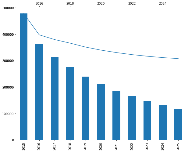
It’s important to remember that a dollar ten years from now is not worth the same as a dollar today. That’s why we need to discount all of the forecasted revenues. I’ll be setting the discount rate at 10% and computing the discount rates for the next 10 years, from 2016 to 2025. We don’t need to discount the revenues of 2015, since it’s supposed to be the present. The formula for this is: \((1 + \text{discount rate})^{-y}\), where \(y\) is the number of years until the revenue is received, and times \(-1\) to say that it is a quotient - a discount.
# Create a discount factor
discount_rate = 0.10
discount = 1 / ((1 + discount_rate) ** np.arange(0,11))
print(discount)
[1.         0.90909091 0.82644628 0.7513148  0.68301346 0.62092132
 0.56447393 0.51315812 0.46650738 0.42409762 0.38554329]
In the first year, we don’t need to discount anything because that’s today’s money worth in today’s dollars. However, after the first year, a dollar would only be worth $0.90, then $0.82, and so on. After ten years, a dollar will only be worth $0.38.
Now if we multiply yearly_revenues by the discount rates, we get the true value of each forecasted revenue in today’s dollars.
# Compute discounted yearly revenue
# Future revenues in todays money
disc_yearly_revenue = yearly_revenue.multiply(discount)
print(disc_yearly_revenue.round(0))
2015   478,414.00
2016   361,460.00
2017   313,800.00
2018   275,110.00
2019   239,911.00
2020   210,936.00
2021   186,527.00
2022   165,596.00
2023   147,671.00
2024   132,083.00
2025   118,581.00
dtype: float64
As we can see above, the $307,568 in 2025 is equivalent to $118,000 in today’s money, which makes a big difference. It’s important to remember that money you’ll receive in the future is worth less than money you receive today. Only by discounting future revenues, we can compare them to today’s acquisition costs and see if it’s a good investment. Indeed, discounting adjusts the value of money received or paid in the future to its present value. So even though a future revenue may seem high, it may not be worth as much as it seems when considering the time value of money. Therefore, always remember to discount future dollars!
When we plot these figures, we can see that the discounted revenue is high in the beginning and then drops dramatically as the years go by, since the further away in the future you get, the less worth the revenue is in today’s dollars.
ax1 = disc_yearly_revenue.plot(kind='bar')
ax2 = ax1.twiny()
yearly_revenue.plot(kind='line', ax=ax2)
Conclusion
In summary, CLV analysis is a critical aspect for any retailer to understand and implement in order to gain a competitive advantage in today’s overcrowded marketplace. By capturing and evaluating CLV, you can determine how much to spend on acquiring new customers, identify and target top future customers, minimize spending on unprofitable ones, and/or build more sustainable and beneficial relationships with your customer base. After all, only by understanding your customers’ buying behaviors, preferences, and concerns can you design more targeted marketing campaigns, personalize your value-added services, and thus improve overall satisfaction and retention.
Now, aside from being an incredibly important metric for retailers, CLV analysis is relatively easy to integrate into your daily operations thanks to the availability of customer’s data and the digital transformation taking place right now. In fact, any serious Customer Relationship Management (CRM) software or e-commerce system already has CLV metrics built in, so you don’t even have to implement them yourself. As such, this tutorial wasn’t only about how to implement CLV, but rather about understanding how it fundamentally works and the competitive advantages it can bring to your business.
That said, CLV can only deliver those benefits once you stop limiting yourself to short-term transactions and shift your marketing strategies to a customer-centric approach based on building sustainable relationships with your customer base.
References
- Netzer, Oded & Lattin, James. (2008). A Hidden Markov Model of Customer Relationship Dynamics. Marketing Science. 27. 10.1287/mksc.1070.0294.
- Lilien, Gary L, Arvind Rangaswamy, and Arnaud De Bruyn. 2017. Principles of Marketing Engineering and Analytics. State College, PA: Decisionpro.
- Grönroos, Christian. 1991. “The Marketing Strategy Continuum: Towards a MarketingConcept for the 1990s.” Management Decision 29 (1). https://doi.org/10.1108/00251749110139106.
- Tarokh, MohammadJafar, and Mahsa EsmaeiliGookeh. n.d. “A New Model to Speculate CLV Based on Markov Chain Model,” 19.
- Bendle, Neil T., and Charan K. Bagga. 2017. “The Confusion About CLV in Case-Based Teaching Materials.” Marketing Education Review 27 (1): 27–38. https://doi.org/10.1080/10528008.2016.1255561.
- Pfeifer, Phillip E., and Robert L. Carraway. 2000. “Modeling Customer Relationships as Markov Chains.” Journal of Interactive Marketing 14 (2): 43–55. https://doi.org/10.1002/(SICI)1520-6653(200021)14:2<43::AID-DIR4>3.0.CO;2-H.
- Arnaud De Bruyn. Foundations of marketing analytics (MOOC). Coursera.
- Dataset from Github repo. Accessed 15 December 2021.
Business Analytics Tutorial RFM Analysis CLV 