Customer Segmentation and Profiling: A Managerial Approach

Introduction

In our previous tutorial on RFM analysis, we let the data speak for itself. We used hierarchical clustering to discover natural groupings in customer behavior, allowing statistical patterns to emerge without imposing our assumptions. That approach revealed four distinct segments: loyal customers, those needing attention, high-value customers at risk, and the truly lost.

But here’s the thing: statistical segmentation isn’t the only game in town, and it’s often not even the most practical one. Today we’re exploring the other side of the coin: managerial segmentation, where experienced business leaders make deliberate choices about how to divide their market based on specific strategic objectives.

Market segmentation sits at the heart of modern marketing. The fundamental insight is simple yet powerful: treating all customers the same way guarantees mediocrity. You can’t offer everyone identical products at identical prices with identical messaging and expect optimal results. Different customers have different needs, different budgets, different buying patterns. Segmentation helps you match your approach to these differences.

The question isn’t whether to segment, but how. The approach you choose should reflect what you’re trying to achieve. If you’re worried about customer churn, you might segment by recency. If you’re planning a premium product launch, you might segment by spending levels. If you’re concerned about price sensitivity ahead of a price increase, that becomes your segmentation basis.

Two Philosophies of Segmentation

Segmentation approaches fall into two broad categories. Post-hoc (or exploratory) segmentation, like the hierarchical clustering we explored last time, discovers patterns you didn’t know existed. You feed the algorithm your data and see what groupings emerge. This approach can reveal surprising insights and challenge your assumptions about your customer base.

A priori (or prescriptive) segmentation works differently. Here, managers proactively choose the segmentation variables based on specific business decisions they’re facing. The segments are defined upfront according to business logic, then customers are assigned to them. This is managerial segmentation, and it’s what most companies actually use in practice.

Why would you choose the simpler approach over sophisticated algorithms? Several reasons. Managerial segmentation is transparent and explainable to stakeholders. It’s easy to implement and maintain without a data science team. It aligns directly with business decisions because you built it around those decisions. And perhaps most importantly, it’s fast. You can create new segments as business needs change without waiting for models to retrain.

The downside is that you might miss patterns that aren’t obvious to human judgment. You’re limited by what you already know or suspect about your customers. This is why the best practice often combines both approaches: use statistical methods to discover patterns and validate assumptions, then implement simple rule-based segments for day-to-day operations.

Defining Our Segmentation Goal

For this tutorial, we want to predict which customers are most likely to purchase again in the near future. This isn’t an academic exercise. Understanding purchase likelihood drives crucial decisions about where to invest your marketing budget. Should you spend money trying to reactivate customers who bought three years ago? Or focus those resources on customers who bought last month and are primed to return?

Recency provides our foundation because it captures purchase likelihood elegantly. Someone who bought from your store three weeks ago exists in a fundamentally different state than someone whose last purchase was three years ago. The recent buyer remembers your brand, recently found value in your products, and likely still has the need that drove their purchase. The distant buyer might have forgotten you, switched to competitors, or moved on from that category entirely.

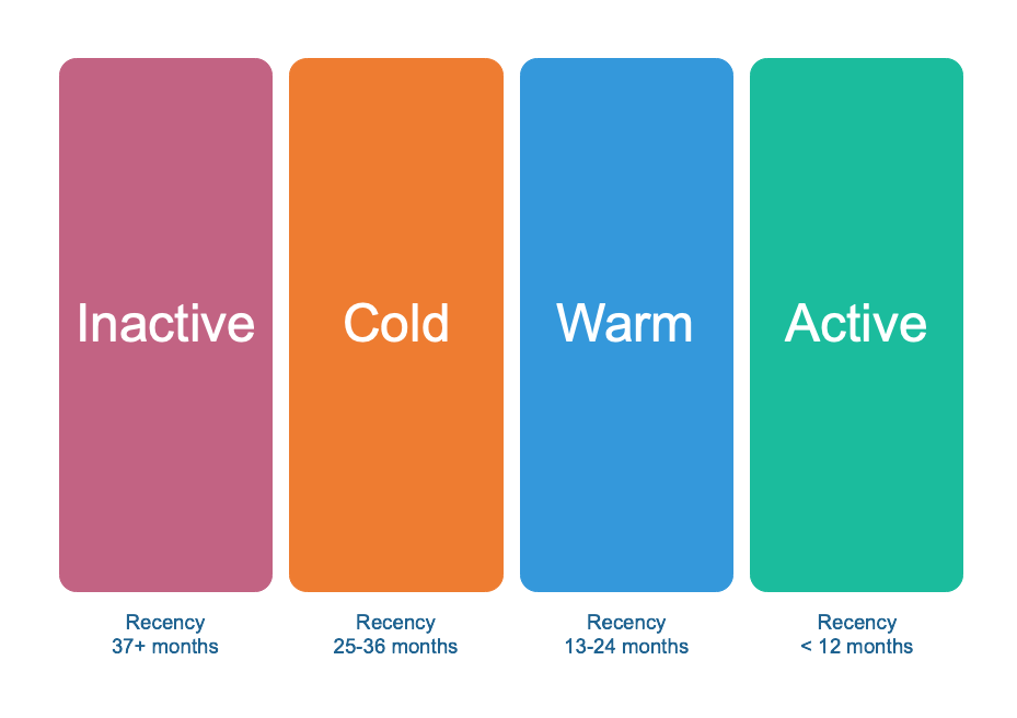
Let’s build our segmentation framework starting with four basic groups based on recency:

Active customers made their last purchase within 12 months. They’re engaged, they know your brand, and they’re likely to buy again soon. These customers are in your active consideration set.

Warm customers last purchased between 13 and 24 months ago. They’re not lost yet, but they’re cooling off. They might be buying from competitors, or life circumstances might have changed. These customers need reengagement before they slip further away.

Cold customers haven’t purchased in 25 to 36 months. The relationship has grown distant. Winning them back requires more aggressive interventions and might not be cost-effective for lower-value customers.

Inactive customers haven’t bought anything in over three years. These customers are essentially lost. Unless they were extremely high-value, the cost of reactivation typically exceeds the likely return.

This four-segment model gives us a starting framework. But a single variable rarely captures enough nuance for effective marketing decisions. We’re leaving money on the table if we treat all active customers the same way, regardless of whether they spend $20 per purchase or $200.

Enriching the Model with RFM

Now we add two more dimensions: frequency and monetary value. This transforms our simple recency-based model into something more sophisticated without becoming unmanageably complex.

We want to identify new customers separately because they require different treatment. Someone who just made their first purchase last month shouldn’t be grouped with loyal customers who’ve been buying for years. The new customer needs cultivation and a positive second-purchase experience. The experienced customer might be ready for higher-tier products or loyalty rewards.

We also want to distinguish between high-value and low-value customers within our active and warm segments. A customer who averages $150 per purchase deserves more personalized attention than someone averaging $25. The marketing spend required to maintain that high-value relationship pays for itself. For the low-value customer, automated campaigns might be more cost-effective.

This thinking leads us to eight segments total:

Within our inactive and cold customers, we maintain single segments. These customers are too far gone or too expensive to subdivide further for most businesses.

Within our warm segment, we create three groups: new warm customers (first purchase 13-24 months ago), warm low-value customers (average spending under $100), and warm high-value customers (average spending $100 or more).

Within our active segment, we mirror this structure: new active customers (first purchase within 12 months), active low-value customers (under $100 average), and active high-value customers ($100+ average).

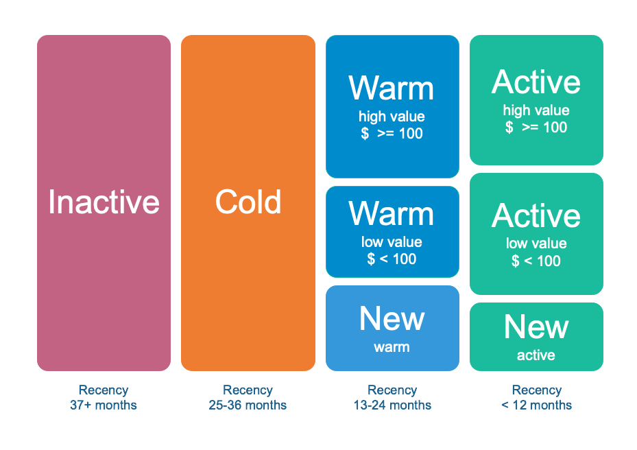
The $100 threshold isn’t arbitrary. Looking at our data distribution from the previous analysis, we saw that 75% of customers spend less than $50 on average, while the top performers spend several hundred dollars. The $100 mark sits in that upper tier where customers demonstrate substantially different value potential. In your business, this threshold might be $50 or $500, depending on your average order values and margin structure.

Similarly, the 12-month window for “active” reflects typical retail repurchase cycles. For some businesses (grocery stores, coffee shops), this might be weeks. For others (furniture, cars), it might be years. Adjust these thresholds to match your industry’s natural buying rhythms.

Building the Segmentation in Python

Let’s implement this framework with the same dataset we used in our previous tutorial. We have 51,243 transactions from 18,417 unique customers spanning January 2005 through December 2015.

# Load required libraries
import numpy as np
import pandas as pd
import matplotlib.pyplot as plt
import squarify
from tabulate import tabulate

# Set up our environment
pd.options.display.float_format = '{:,.2f}'.format
plt.rcParams["figure.figsize"] = (12, 8)

# Load the dataset
columns = ['customer_id', 'purchase_amount', 'date_of_purchase']
df = pd.read_csv('purchases.txt', header=None, sep='\t', names=columns)

# Quick look at sample records
df.sample(n=5, random_state=57)

       customer_id  purchase_amount  date_of_purchase
4510          8060            30.00        2014-12-24
17761        109180            50.00        2009-11-25
39110          9830            30.00        2007-06-12
37183         56400            60.00        2009-09-30
33705         41290            60.00        2007-08-21

The data looks clean and ready to work with. Now we prepare our time-based calculations:

# Convert dates to datetime objects
df['date_of_purchase'] = pd.to_datetime(df['date_of_purchase'], format='%Y-%m-%d')

# Extract year for potential cohort analysis
df['year_of_purchase'] = df['date_of_purchase'].dt.year

# Calculate days since each purchase (using Jan 1, 2016 as reference)
basedate = pd.Timestamp('2016-01-01')
df['days_since'] = (basedate - df['date_of_purchase']).dt.days

# Check our work
df.info()

<class 'pandas.core.frame.DataFrame'>
RangeIndex: 51243 entries, 0 to 51242
Data columns (total 5 columns):
 #   Column            Non-Null Count  Dtype         
---  ------            --------------  -----         
 0   customer_id       51243 non-null  int64         
 1   purchase_amount   51243 non-null  float64       
 2   date_of_purchase  51243 non-null  datetime64[ns]
 3   year_of_purchase  51243 non-null  int64         
 4   days_since        51243 non-null  int64         
dtypes: datetime64[ns](1), float64(1), int64(3)
memory usage: 2.0 MB

Perfect. Everything is properly typed and ready for analysis.

Computing RFM Metrics

Now we aggregate our transaction-level data into customer-level metrics. For each customer, we need three values: how recently they purchased (minimum days since), how frequently they purchase (count of transactions), and how much they typically spend (average purchase amount).

We also want to track when each customer made their first purchase. This helps us identify truly new customers versus those who are simply returning after a long absence.

# Calculate RFM metrics using native pandas
customers = df.groupby('customer_id').agg({
    'days_since': ['min', 'max'],       # Min = recency, Max = first purchase
    'customer_id': 'count',              # Count = frequency
    'purchase_amount': 'mean'            # Mean = average spending
})

# Flatten column names and rename for clarity
customers.columns = ['recency', 'first_purchase', 'frequency', 'amount']
customers = customers.reset_index()

# Display summary statistics
print(tabulate(customers.describe(), headers='keys', tablefmt='psql', floatfmt='.2f'))

+-------+---------------+-----------+------------------+-------------+----------+
|       | customer_id   | recency   | first_purchase   | frequency   | amount   |
|-------+---------------+-----------+------------------+-------------+----------|
| count | 18417.00      | 18417.00  | 18417.00         | 18417.00    | 18417.00 |
| mean  | 137574.24     | 1253.04   | 1984.01          | 2.78        | 57.79    |
| std   | 69504.61      | 1081.44   | 1133.41          | 2.94        | 154.36   |
| min   | 10.00         | 1.00      | 1.00             | 1.00        | 5.00     |
| 25%   | 81990.00      | 244.00    | 988.00           | 1.00        | 21.67    |
| 50%   | 136430.00     | 1070.00   | 2087.00          | 2.00        | 30.00    |
| 75%   | 195100.00     | 2130.00   | 2992.00          | 3.00        | 50.00    |
| max   | 264200.00     | 4014.00   | 4016.00          | 45.00       | 4500.00  |
+-------+---------------+-----------+------------------+-------------+----------+

These statistics tell important stories. The median customer last purchased 1,070 days ago (nearly three years), has made only two purchases total, and averages $30 per transaction. This is why segmentation matters. That median customer probably needs different treatment than the customer who made 45 purchases averaging $4,500 each.

Let’s look at the first few customers:

print(tabulate(customers.head(), headers='keys', tablefmt='psql', floatfmt='.2f'))

+----+---------------+-----------+------------------+-------------+----------+
|    | customer_id   | recency   | first_purchase   | frequency   | amount   |
|----+---------------+-----------+------------------+-------------+----------|
|  0 | 10            | 3829.00   | 3829.00          | 1.00        | 30.00    |
|  1 | 80            | 343.00    | 3751.00          | 7.00        | 71.43    |
|  2 | 90            | 758.00    | 3783.00          | 10.00       | 115.80   |
|  3 | 120           | 1401.00   | 1401.00          | 1.00        | 20.00    |
|  4 | 130           | 2970.00   | 3710.00          | 2.00        | 50.00    |
+----+---------------+-----------+------------------+-------------+----------+

Customer 90 stands out immediately. Ten purchases averaging $115.80, with the last one 758 days ago. That’s a valuable customer who’s gone quiet. Understanding why customers like this stop buying becomes strategically important.

Let’s visualize the distributions of our RFM variables:

# Create histogram grid for RFM variables
customers.iloc[:, 1:].hist(bins=30, figsize=(15, 10))
plt.tight_layout()
plt.savefig('rfm_distributions.png', dpi=150, bbox_inches='tight')
plt.show()

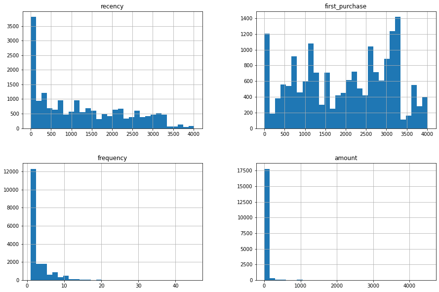
The distributions reveal the same patterns we saw in our clustering analysis. Recency spreads relatively evenly with a spike of recent activity. Frequency is heavily right-skewed with most customers making few purchases. The monetary distribution clusters in the low range with a long tail of high spenders. These patterns justify our decision to create distinct high-value and low-value segments.

Building the Four-Segment Base Model

We start with the simplest version: segmenting purely on recency. This foundation helps us understand the basic health of our customer base before we add complexity.

The segmentation logic proceeds from most distant to most recent. We identify inactive customers first (those who haven’t purchased in over three years), then work our way forward through cold, warm, and finally active customers.

# Initialize segment column
customers['segment'] = None

# Segment 1: Inactive (more than 3 years since last purchase)
customers.loc[customers['recency'] > 365*3, 'segment'] = 'inactive'

# Segment 2: Cold (2-3 years since last purchase)
customers.loc[(customers['recency'] <= 365*3) & 
              (customers['recency'] > 365*2), 'segment'] = 'cold'

# Segment 3: Warm (1-2 years since last purchase)
customers.loc[(customers['recency'] <= 365*2) & 
              (customers['recency'] > 365), 'segment'] = 'warm'

# Segment 4: Active (less than 1 year since last purchase)
customers.loc[customers['recency'] <= 365, 'segment'] = 'active'

# Count customers in each segment
segment_counts = customers['segment'].value_counts()
print(segment_counts)

inactive    9158
active      5398
warm        1958
cold        1903
Name: segment, dtype: int64

These numbers reveal a troubling pattern. Nearly half our customer base (9,158 out of 18,417) hasn’t purchased in over three years. They’re effectively lost. Another 1,903 customers are cold and at serious risk. That’s 11,061 customers (60% of the total) who are either gone or going.

On the positive side, we have 5,398 active customers and 1,958 warm customers still in play. These 7,356 customers represent our real opportunity. They’re still engaged or recently engaged, and interventions with them are likely to be cost-effective.

Before moving forward, we need to understand why so many customers became inactive. This requires deeper investigation: reviewing customer service records, analyzing product quality issues, benchmarking competitor offerings, and potentially surveying lost customers. Understanding the causes of churn must precede any reactivation strategy. Throwing marketing dollars at inactive customers without addressing root causes wastes money.

Let’s visualize the segment sizes:

# Create treemap visualization
plt.figure(figsize=(10, 6))
plt.rcParams.update({'font.size': 18})

squarify.plot(
    sizes=segment_counts,
    label=segment_counts.index,
    color=['#9b59b6', '#2ecc71', '#3498db', '#e67e22'],
    alpha=0.6,
    text_kwargs={'fontsize': 16, 'weight': 'bold'}
)
plt.title('Customer Segments by Recency', fontsize=20, pad=20)
plt.axis('off')
plt.tight_layout()
plt.savefig('four_segments_treemap.png', dpi=150, bbox_inches='tight')
plt.show()

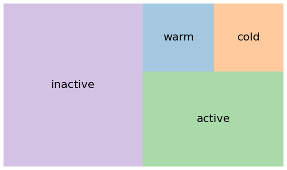
The treemap makes the imbalance viscerally clear. That massive purple block of inactive customers dominates the visualization. This is your wake-up call about customer retention. Every business loses customers, but losing 50% to inactivity suggests systematic problems worth investigating.

Expanding to Eight Segments

The four-segment model provides a foundation, but it treats all active customers identically. A customer who made their first purchase two weeks ago receives the same classification as someone who’s been buying regularly for five years. A customer spending $25 per order gets grouped with someone spending $250. We’re leaving strategic opportunities on the table.

Let’s add nuance by incorporating frequency and monetary value, focusing on our active and warm segments where marketing investments are most likely to pay off.

We use numpy’s select function to handle the segmentation logic cleanly. This approach avoids the overlapping condition problems that plague sequential if-then statements:

# Define our segmentation conditions and labels
conditions = [
    customers['recency'] > 365*3,
    (customers['recency'] <= 365*3) & (customers['recency'] > 365*2),
    
    # Warm segment subdivisions
    (customers['segment'] == 'warm') & (customers['first_purchase'] <= 365*2),
    (customers['segment'] == 'warm') & (customers['amount'] >= 100),
    (customers['segment'] == 'warm') & (customers['amount'] < 100),
    
    # Active segment subdivisions
    (customers['segment'] == 'active') & (customers['first_purchase'] <= 365),
    (customers['segment'] == 'active') & (customers['amount'] >= 100),
    (customers['segment'] == 'active') & (customers['amount'] < 100)
]

choices = [
    'inactive',
    'cold',
    'new warm',
    'warm high value',
    'warm low value',
    'new active',
    'active high value',
    'active low value'
]

customers['segment'] = np.select(conditions, choices, default=customers['segment'])

# Count customers in each refined segment
refined_counts = customers['segment'].value_counts()
print(refined_counts)

inactive             9158
active low value     3313
cold                 1903
new active           1512
new warm              938
warm low value        901
active high value     573
warm high value       119
Name: segment, dtype: int64

These refined segments tell richer stories. Among our 5,398 active customers, 1,512 are brand new (first purchase within the year). They need welcome campaigns and second-purchase incentives to cement the relationship. Another 3,313 are low-value repeat customers who might respond well to volume discounts or bundles. The 573 high-value active customers are your VIPs who deserve personalized service and exclusive offers.

The warm segment shows similar patterns. We have 938 customers who made their first (and only) purchase 13-24 months ago. They tried once and never came back. That requires investigation. Why didn’t they return? Meanwhile, 901 warm low-value customers need automated reengagement, while the 119 warm high-value customers justify personal outreach.

Let’s create a ordered categorical variable to display these segments logically:

# Create ordered categorical for better sorting and display
segment_order = [
    'inactive', 
    'cold', 
    'warm high value', 
    'warm low value', 
    'new warm',
    'active high value', 
    'active low value', 
    'new active'
]

customers['segment'] = pd.Categorical(
    customers['segment'],
    categories=segment_order,
    ordered=True
)

# Sort by segment for better viewing
customers_sorted = customers.sort_values('segment')

# Display sample from each segment
print("\nFirst 5 customers (inactive segment):")
print(tabulate(
    customers_sorted[['customer_id', 'segment']].head(),
    headers='keys',
    tablefmt='psql',
    showindex=False
))

print("\nLast 5 customers (new active segment):")
print(tabulate(
    customers_sorted[['customer_id', 'segment']].tail(),
    headers='keys',
    tablefmt='psql',
    showindex=False
))

First 5 customers (inactive segment):
+---------------+------------+
| customer_id   | segment    |
|---------------+------------|
| 10            | inactive   |
| 119690        | inactive   |
| 119710        | inactive   |
| 119720        | inactive   |
| 119730        | inactive   |
+---------------+------------+

Last 5 customers (new active segment):
+---------------+--------------+
| customer_id   | segment      |
|---------------+--------------|
| 252380        | new active   |
| 252370        | new active   |
| 252360        | new active   |
| 252450        | new active   |
| 264200        | new active   |
+---------------+--------------+

Now let’s visualize the complete eight-segment model:

# Create color scheme that groups related segments
colors = [
    '#9b59b6',  # inactive - purple
    '#e67e22',  # cold - orange
    '#3498db',  # warm high value - blue
    '#2ecc71',  # warm low value - green
    '#3498db',  # new warm - blue
    '#3498db',  # active high value - blue
    '#2ecc71',  # active low value - green
    '#3498db'   # new active - blue
]

plt.figure(figsize=(16, 10))
plt.rcParams.update({'font.size': 14})

squarify.plot(
    sizes=refined_counts.reindex(segment_order),
    label=segment_order,
    color=colors,
    alpha=0.6,
    pad=True,
    text_kwargs={'fontsize': 13, 'weight': 'bold'}
)
plt.title('Eight-Segment RFM Customer Model', fontsize=20, pad=20)
plt.axis('off')
plt.tight_layout()
plt.savefig('eight_segments_treemap.png', dpi=150, bbox_inches='tight')
plt.show()

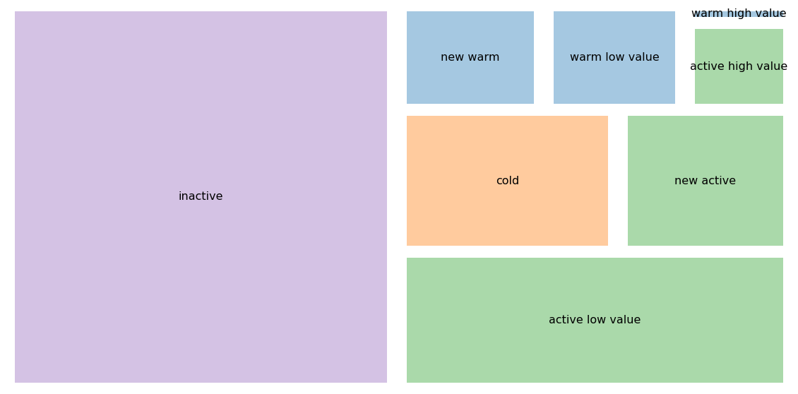
The color coding helps group related segments. Blue shades indicate higher engagement or value segments worth significant investment. Green shows lower-value but still active relationships. Orange represents customers at risk. Purple marks those who are lost.

Creating Buyer Personas

Numbers and segments are useful for analysis, but marketing teams need something more tangible to guide their campaigns. This is where buyer personas come in. A persona transforms abstract segment characteristics into a concrete, relatable character that represents the typical customer in that segment.

Creating effective personas requires moving beyond pure statistics. You synthesize the quantitative data (average purchase frequency, spending levels, recency) with qualitative insights from customer interviews, support interactions, and behavioral observations. The goal is a semi-fictional character that embodies the needs, motivations, and behaviors of customers in each segment.

For example, your “active high value” segment might become “Premium Paula,” a 35-45 year old professional who values quality over price, makes frequent purchases of $150-300, and expects excellent customer service. She’s time-poor but financially comfortable. Your marketing to Paula emphasizes convenience, exclusivity, and premium features rather than discounts.

Your “new active” segment might be “First-Timer Frank,” a 25-35 year old who just made his first purchase after clicking a Facebook ad. He’s price-conscious, comparing alternatives carefully, and highly susceptible to buyer’s remorse. Frank needs reassurance about his purchase decision and gentle nudges toward a second purchase through targeted follow-up campaigns.

The persona approach works because it makes segmentation memorable and actionable. Marketing teams can ask “What would Paula want from this campaign?” or “How would Frank respond to this offer?” These questions produce better, more targeted strategies than abstract references to “Segment 6.”

Building comprehensive personas requires data beyond what we have in this transaction dataset. You need demographic information, psychographic profiles, purchase motivations, and pain points. Customer surveys, interviews, and behavioral analytics all contribute. The RFM segmentation provides the behavioral foundation, but personas flesh out the complete customer picture.

Strategic Implications for Each Segment

Understanding the segments means nothing without actionable strategies. Let’s walk through what each segment needs and how to approach them:

Inactive customers are essentially lost. For most businesses, the cost of reactivation exceeds the likely return unless these customers were previously very high-value. Your best strategy here is often to stop spending money on them. Remove them from expensive marketing campaigns. If you must try reactivation, make it low-cost and automated. Accept that most won’t return and focus your energy elsewhere.

Cold customers require triage. Analyze their historical value. High-value cold customers might justify personalized outreach: a phone call, a special offer, a survey to understand what went wrong. Low-value cold customers get automated “we miss you” campaigns at most. The key decision is whether the expected recovery value exceeds the intervention cost.

Warm low-value customers need efficient reengagement. Automated email campaigns work well here. Remind them what they previously bought and suggest related products. Offer time-limited discounts to create urgency. Use dynamic content that personalizes at scale without manual effort. These campaigns should be cheap to execute because individual customer value is modest.

Warm high-value customers deserve personal attention. Someone in your company should reach out directly. Understand why they stopped buying. Address any product or service issues. Offer them exclusive early access to new products or special pricing. A small investment in personal outreach can recover substantial customer lifetime value.

New warm customers represent a special challenge. They bought once and never returned. This might mean the first purchase disappointed them, or they never intended to become repeat customers. Send a survey asking about their experience. Offer a compelling reason to give you a second chance. If they don’t respond, let them fade into cold status rather than wasting resources.

Active low-value customers are your bread and butter. Keep them engaged with regular communications about new products and promotions. Encourage larger basket sizes through bundles and volume discounts. Consider loyalty programs that reward frequency. The goal is to gradually increase their lifetime value through sustained, low-cost engagement.

Active high-value customers are your champions. Give them white-glove treatment. Offer exclusive products or early access. Create VIP programs with special perks. Ask for referrals. Feature them in case studies (with permission). These customers can become brand advocates who generate new customer acquisition through word-of-mouth. Never take them for granted.

New active customers are in a critical window. Their second purchase is the most important moment in the customer relationship. Send welcome campaigns that educate them about your full product range. Offer second-purchase incentives. Solicit feedback. Make them feel valued and appreciated. Converting new customers into repeat customers is often cheaper than acquiring entirely new customers.

Comparing Statistical and Managerial Approaches

Our hierarchical clustering analysis from the previous tutorial and this managerial segmentation both produced actionable customer groups, but through fundamentally different paths. Understanding when to use each approach helps you make smarter segmentation decisions.

Statistical clustering discovered patterns we didn’t specify in advance. The algorithm found that some customers were loyal (high frequency, recent purchases), while others were high-value but lapsed. These insights emerged from the data itself. The downside was complexity: hierarchical clustering requires data preparation, distance calculations, and decisions about cutting dendrograms. Explaining it to non-technical stakeholders takes effort.

Managerial segmentation implements business logic directly. If you know that recency predicts purchase likelihood and that high-value customers deserve different treatment, you can code that logic in an afternoon. Everyone understands the rules. The approach is transparent and easily adjusted as business needs change. The downside is that you might miss non-obvious patterns or impose assumptions that don’t match reality.

The best practice combines both. Use statistical methods periodically to discover patterns, validate assumptions, and challenge your thinking. Maybe clustering reveals that three purchases is the magic threshold where loyalty really kicks in, or that spending over $75 predicts dramatically different behavior than spending $74. These insights then inform the rules you set up for ongoing managerial segmentation.

For operational deployment, managerial segmentation often wins. It runs fast, updates easily, and requires no special infrastructure. Your marketing automation platform can implement it directly. You don’t need a data science team to maintain it. This is why most companies use rule-based segmentation for day-to-day operations even if they periodically validate those rules with more sophisticated analysis.

The Exploration-Exploitation Balance

One risk of managerial segmentation is strategic stagnation. When managers define segments based on experience and judgment, they tend to implement familiar strategies. The approach works, but it rarely surprises you. You’re exploiting what you already know rather than exploring what you might discover.

This tension between exploration and exploitation appears throughout business strategy. Do you stick with proven approaches that generate reliable results? Or do you experiment with new ideas that might fail but could also produce breakthrough insights? Both are necessary. Pure exploitation leaves you vulnerable when markets shift. Pure exploration wastes resources on untested ideas.

In segmentation specifically, this means periodically challenging your managerial segments with data-driven analysis. Run clustering once per year to see if your customer base has shifted. Test whether your thresholds still make sense. Survey customers to validate that your persona assumptions remain accurate. The goal isn’t to constantly redesign your segmentation, but to ensure your existing approach remains grounded in reality.

Research in cognitive neuroscience shows that the capacity for exploration and learning new patterns doesn’t necessarily decline with age or experience, provided people remain open to learning and engage in deliberate practice. Experienced managers can innovate, but it requires conscious effort to question assumptions and test alternatives. Creating space for periodic data-driven exploration helps maintain that innovative capacity.

Practical Implementation Considerations

When you implement segmentation in production systems, several practical issues emerge beyond the analytical framework. Your customer database updates constantly as new purchases occur. Customers move between segments. Your segmentation code needs to run automatically on schedule, updating segment assignments without manual intervention.

Integration with marketing automation platforms becomes critical. The segments you define need to flow into your email marketing system, CRM, and advertising platforms. This requires APIs, data pipelines, and careful data governance to ensure consistency across systems. A customer shouldn’t receive a “new customer” campaign in one channel while getting a “loyal customer” message in another.

Seasonal effects can distort your segments. A customer who looks inactive in February might simply buy holiday gifts in December. Understanding your business’s natural purchase cycles helps you set appropriate recency thresholds and interpret segment changes. You might need different segmentation rules for different product categories if they have distinct purchase patterns.

Validation and monitoring matter. Track how segment composition changes over time. Monitor whether your marketing campaigns achieve different results across segments as expected. If your “active high value” customers don’t respond better than “active low value” customers, something is wrong with either the segmentation or the targeting. Continuous measurement keeps your segmentation relevant and effective.

Conclusion

Managerial segmentation offers a practical, transparent approach to dividing your customer base into actionable groups. By focusing on the business decisions you need to make and the variables that drive those decisions, you create segments that directly support strategy execution. The approach is simple enough to explain to any stakeholder, fast enough to update frequently, and flexible enough to adapt as business needs evolve.

We started with a basic recency-based model that revealed the stark reality of customer retention: 50% of customers had become inactive. We then enriched this model with frequency and monetary dimensions, creating eight segments that capture the nuance of customer value and engagement. Each segment suggests specific marketing strategies matched to customer state and potential.

The power of this approach lies not in algorithmic sophistication but in business alignment. When your segmentation directly reflects the decisions you’re trying to make (who to target, how much to invest, what message to send), implementation becomes straightforward. Marketing teams understand the logic. IT teams can automate the rules. Executives can track segment composition as a business metric.

But managerial segmentation works best when informed by periodic statistical exploration. Use clustering and other analytical techniques to validate your assumptions, discover patterns you might have missed, and challenge your thinking. Then translate those insights into simple rules that your organization can execute at scale.

The goal isn’t perfect segmentation. The goal is actionable segmentation that improves resource allocation and customer outcomes. Whether you achieve that through sophisticated algorithms or simple business rules matters less than whether your segmentation drives better decisions. Often, the simplest approach that your organization can actually implement beats the most elegant solution that never makes it into production.

In our two tutorials, we’ve explored both ends of the segmentation spectrum: data-driven discovery through hierarchical clustering and business-driven prescription through managerial rules. Master both approaches, understand their strengths and limitations, and choose the right tool for each situation. That’s the mark of sophisticated customer analytics.

References

1. Lilien, Gary L, Arvind Rangaswamy, and Arnaud De Bruyn. 2017. Principles of Marketing Engineering and Analytics. State College, PA: DecisionPro.

2. Piercy, Nigel F., and Neil A. Morgan. 1993. “Strategic and Operational Market Segmentation: A Managerial Analysis.” Journal of Strategic Marketing 1 (2): 123-40. https://doi.org/10.1080/09652549300000008.

3. Wind, Yoram. 1978. “Issues and Advances in Segmentation Research.” Journal of Marketing Research 15 (3): 317-34. https://doi.org/10.2307/3150580.

4. Armstrong, G.M., S. Adam, S.M. Denize, M. Volkov, and P. Kotler. 2017. Principles of Marketing. Pearson Australia.

5. Laureiro-Martínez, Daniella, Stefano Brusoni, Nicola Canessa, and Maurizio Zollo. 2015. “Understanding the Exploration-Exploitation Dilemma: An fMRI Study of Attention Control and Decision-Making Performance.” Strategic Management Journal 36 (3): 319-38. https://doi.org/10.1002/smj.2221.

6. Arnaud De Bruyn. Foundations of Marketing Analytics (MOOC). Coursera.

7. Dataset from Github repo. Accessed 15 December 2021.