Forecasting Customer Lifetime Value Using RFM-Analysis and Markov Chain
Introduction
Customer Lifetime Value (CLV) quantifies the total present value of all future cash flows from a customer relationship. It transforms customer analytics from describing the past to valuing the future.
In our first tutorial, we segmented customers using hierarchical clustering. The second tutorial implemented managerial segmentation with business rules. Our third tutorial built models that forecast next-period purchase probability and spending.
Today we forecast customer value over multiple years using Markov chain modeling. We’ll capture how customers migrate between segments over time, project future revenue streams, and discount them to present value.
Why CLV Matters
Acquiring new customers costs five to twenty-five times more than retaining existing ones. You can’t treat a customer who will generate $5,000 over five years the same as one who will generate $50. Without CLV, you can’t make these distinctions rationally.
The Business Case
Consider: your acquisition campaign costs $100,000 and brings 500 new customers generating $120,000 in immediate revenue. Looks profitable. But if discount-driven customers generate only $150 in lifetime value while full-price customers generate $800, the campaign might actually destroy value. CLV reveals the true economics.
CLV guides decisions across the business: acquisition channel comparison, optimal acquisition spending, retention investment prioritization, and product development focus.
Markov Chain Migration Models
Our approach uses a migration model based on Markov chains. By comparing customer segments from consecutive years, we see how customers moved between segments. Each transition has a probability we can estimate from historical data. These transition probabilities form a matrix.
Once you have this transition matrix, you can project it forward indefinitely. Multiply today’s distribution by the transition matrix to get next year’s. Keep going to project five or ten years forward.
The key assumption is that the process is memoryless: future transitions depend only on the current segment, not the path that led there. We also assume no new customer acquisition in our projections (we’re valuing the existing customer base only).
Building the Analysis in Python
Let’s implement this framework using our familiar dataset. We’ll reuse the segmentation functions we developed in the previous tutorial to keep our code clean and maintainable.
# Import required libraries
import matplotlib.pyplot as plt
import numpy as np
import pandas as pd
import squarify
from tabulate import tabulate

# Set up environment
pd.options.display.float_format = '{:,.2f}'.format
plt.rcParams["figure.figsize"] = (12, 8)

# Load the dataset
columns = ['customer_id', 'purchase_amount', 'date_of_purchase']
df = pd.read_csv('purchases.txt', header=None, sep='\t', names=columns)

# Convert to datetime and create time-based features
df['date_of_purchase'] = pd.to_datetime(df['date_of_purchase'], format='%Y-%m-%d')
df['year_of_purchase'] = df['date_of_purchase'].dt.year

# Set reference date for calculating recency
basedate = pd.Timestamp('2016-01-01')
df['days_since'] = (basedate - df['date_of_purchase']).dt.days
Now we’ll use our reusable functions from the previous tutorial to calculate RFM and segment customers:
def calculate_rfm(dataframe, reference_date=None, days_lookback=None):
    """
    Calculate RFM metrics for customers.

    Parameters:
    -----------
    dataframe : DataFrame
        Transaction data with customer_id, purchase_amount, days_since
    days_lookback : int, optional
        Only consider transactions within this many days (default: None, uses all)

    Returns:
    --------
    DataFrame with customer_id and RFM metrics
    """
    if days_lookback is not None:
        df_filtered = dataframe[dataframe['days_since'] > days_lookback].copy()
        df_filtered['days_since'] = df_filtered['days_since'] - days_lookback
    else:
        df_filtered = dataframe.copy()

    rfm = df_filtered.groupby('customer_id').agg({
        'days_since': ['min', 'max'],
        'customer_id': 'count',
        'purchase_amount': ['mean', 'max']
    })

    rfm.columns = ['recency', 'first_purchase', 'frequency', 'avg_amount', 'max_amount']
    rfm = rfm.reset_index()

    return rfm


def segment_customers(rfm_data):
    """
    Segment customers based on RFM metrics using managerial rules.
    """
    customers = rfm_data.copy()

    conditions = [
        customers['recency'] > 365 * 3,
        (customers['recency'] <= 365 * 3) & (customers['recency'] > 365 * 2),
        (customers['recency'] <= 365 * 2) & (customers['recency'] > 365) &
            (customers['first_purchase'] <= 365 * 2),
        (customers['recency'] <= 365 * 2) & (customers['recency'] > 365) &
            (customers['avg_amount'] >= 100),
        (customers['recency'] <= 365 * 2) & (customers['recency'] > 365) &
            (customers['avg_amount'] < 100),
        (customers['recency'] <= 365) & (customers['first_purchase'] <= 365),
        (customers['recency'] <= 365) & (customers['avg_amount'] >= 100),
        (customers['recency'] <= 365) & (customers['avg_amount'] < 100)
    ]

    choices = [
        'inactive',
        'cold',
        'new warm',
        'warm high value',
        'warm low value',
        'new active',
        'active high value',
        'active low value'
    ]

    customers['segment'] = np.select(conditions, choices, default='other')

    segment_order = [
        'inactive', 'cold', 'warm high value', 'warm low value', 'new warm',
        'active high value', 'active low value', 'new active'
    ]
    customers['segment'] = pd.Categorical(
        customers['segment'],
        categories=segment_order,
        ordered=True
    )

    return customers.sort_values('segment')


# Calculate segments for both years
customers_2014 = calculate_rfm(df, days_lookback=365)
customers_2014 = segment_customers(customers_2014)

customers_2015 = calculate_rfm(df)
customers_2015 = segment_customers(customers_2015)

print("2014 Segment Distribution:")
print(customers_2014['segment'].value_counts())
print("\n2015 Segment Distribution:")
print(customers_2015['segment'].value_counts())
2014 Segment Distribution:
inactive             8602
active low value     3094
cold                 1923
new active           1474
new warm              936
warm low value        835
active high value     476
warm high value       108
Name: segment, dtype: int64

2015 Segment Distribution:
inactive             9158
active low value     3313
cold                 1903
new active           1512
new warm              938
warm low value        901
active high value     573
warm high value       119
Name: segment, dtype: int64
Inactive customers grew from 8,602 to 9,158 (churn). Active high value grew from 476 to 573 (customer development). Understanding these flows becomes critical for CLV estimation.
Constructing the Transition Matrix
The transition matrix captures the probability of moving from any segment in 2014 to any segment in 2015. To build it, we need to track individual customer movements across both years:
# Merge 2014 and 2015 segments by customer_id
# Use left join to keep all 2014 customers
transitions_df = customers_2014[['customer_id', 'segment']].merge(
    customers_2015[['customer_id', 'segment']],
    on='customer_id',
    how='left',
    suffixes=('_2014', '_2015')
)

# Handle customers who didn't appear in 2015 data (extremely rare edge case)
# They would have transitioned to inactive
transitions_df['segment_2015'] = transitions_df['segment_2015'].fillna('inactive')

print("\nSample transitions:")
print(tabulate(transitions_df.tail(10), headers='keys', tablefmt='psql', showindex=False))
Sample transitions:
+---------------+----------------+----------------+
| customer_id   | segment_2014   | segment_2015   |
+---------------+----------------+----------------+
| 221470        | new active     | new warm       |
| 221460        | new active     | active low value |
| 221450        | new active     | new warm       |
| 221430        | new active     | new warm       |
| 245840        | new active     | new warm       |
| 245830        | new active     | active low value |
| 245820        | new active     | active low value |
| 245810        | new active     | new warm       |
| 245800        | new active     | active low value |
| 245790        | new active     | new warm       |
+---------------+----------------+----------------+
Now we create the transition matrix using cross-tabulation:
# Create cross-tabulation of transitions (raw counts)
transition_counts = pd.crosstab(
    transitions_df['segment_2014'],
    transitions_df['segment_2015'],
    dropna=False
)

print("\nTransition Counts (2014 → 2015):")
print(transition_counts)
Transition Counts (2014 → 2015):
segment_2015       inactive  cold  warm high value  warm low value  new warm  \
segment_2014
inactive               7227     0                 0               0         0
cold                   1931     0                 0               0         0
warm high value           0    75                 0               0         0
warm low value            0   689                 0               0         0
new warm                  0  1139                 0               0         0
active high value         0     0               119               0         0
active low value          0     0                 0             901         0
new active                0     0                 0               0       938

segment_2015       active high value  active low value
segment_2014
inactive                          35               250
cold                              22               200
warm high value                   35                 1
warm low value                     1               266
new warm                          15                96
active high value                354                 2
active low value                  22              2088
new active                        89               410
Of 8,602 inactive customers in 2014, 7,227 remained inactive (84%). Of 476 active high value, 354 stayed in that segment (74%). The new active segment shows 64% became new warm (didn’t repurchase), highlighting the importance of second-purchase campaigns.
Now we convert counts to probabilities:
# Convert counts to probabilities
transition_matrix = transition_counts.div(transition_counts.sum(axis=1), axis=0)

print("\nTransition Matrix (Probabilities):")
print(transition_matrix.round(3))
Transition Matrix (Probabilities):
segment_2015       inactive   cold  warm high value  warm low value  new warm  \
segment_2014
inactive              0.962  0.000            0.000           0.000     0.000
cold                  0.897  0.000            0.000           0.000     0.000
warm high value       0.000  0.676            0.000           0.000     0.000
warm low value        0.000  0.721            0.000           0.000     0.000
new warm              0.000  0.912            0.000           0.000     0.000
active high value     0.000  0.000            0.251           0.000     0.000
active low value      0.000  0.000            0.000           0.299     0.000
new active            0.000  0.000            0.000           0.000     0.645

segment_2015       active high value  active low value
segment_2014
inactive                       0.005             0.033
cold                           0.010             0.093
warm high value                0.315             0.009
warm low value                 0.001             0.278
new warm                       0.012             0.077
active high value              0.746             0.004
active low value               0.007             0.693
new active                     0.061             0.282
An inactive 2014 customer has a 96.2% chance of staying inactive, 0.5% of becoming active high value, and 3.3% of becoming active low value.
Validating the Transition Matrix
Does multiplying our 2014 distribution by the transition matrix accurately reproduce the actual 2015 distribution?
# Get 2014 segment counts as a vector
segment_2014_counts = customers_2014['segment'].value_counts().reindex(
    transition_matrix.index, fill_value=0
)

# Predict 2015 distribution by matrix multiplication
predicted_2015 = segment_2014_counts.dot(transition_matrix).round(0)

# Get actual 2015 distribution
actual_2015 = customers_2015['segment'].value_counts().reindex(
    transition_matrix.columns, fill_value=0
)

# Compare predictions to actuals
validation = pd.DataFrame({
    '2014_actual': segment_2014_counts,
    '2015_predicted': predicted_2015.astype(int),
    '2015_actual': actual_2015,
    'error': actual_2015 - predicted_2015.astype(int),
    'pct_error': ((actual_2015 - predicted_2015) / actual_2015 * 100).round(1)
})

print("\nTransition Matrix Validation:")
print(tabulate(validation, headers='keys', tablefmt='psql'))
Transition Matrix Validation:
+-------------------+--------------+------------------+---------------+---------+-------------+
| segment           | 2014_actual  | 2015_predicted   | 2015_actual   | error   | pct_error   |
+-------------------+--------------+------------------+---------------+---------+-------------+
| inactive          |     8602.00  |         9212.00  |      9158.00  |  -54.00 |       -0.60 |
| cold              |     1923.00  |         1781.00  |      1903.00  |  122.00 |        6.41 |
| warm high value   |      108.00  |          137.00  |       119.00  |  -18.00 |      -15.13 |
| warm low value    |      835.00  |          931.00  |       901.00  |  -30.00 |       -3.33 |
| new warm          |      936.00  |            0.00  |       938.00  |  938.00 |      100.00 |
| active high value |      476.00  |          552.00  |       573.00  |   21.00 |        3.67 |
| active low value  |     3094.00  |         3292.00  |      3313.00  |   21.00 |        0.63 |
| new active        |     1474.00  |            0.00  |      1512.00  | 1512.00 |      100.00 |
+-------------------+--------------+------------------+---------------+---------+-------------+
Most segments have errors under 7%. Inactive customers predicted at 9,212 vs. actual 9,158 (0.6% error). The new warm and new active segments show 100% error because “new” customers can only enter through acquisition, which our transition matrix doesn’t model.
Projecting Future Segment Evolution
With a validated transition matrix, we can now project customer distribution across future years. We’ll create a matrix where rows represent segments and columns represent years from 2015 through 2025:
# Initialize projection matrix
# Rows = segments, Columns = years
years = np.arange(2015, 2026)
segment_projection = pd.DataFrame(
    0,
    index=customers_2015['segment'].cat.categories,
    columns=years
)

# Populate 2015 with actual counts
segment_projection[2015] = customers_2015['segment'].value_counts().reindex(
    segment_projection.index, fill_value=0
)

# Project forward using matrix multiplication
for year in range(2016, 2026):
    segment_projection[year] = segment_projection[year-1].dot(transition_matrix).round(0)

# Convert to integers (can't have fractional customers)
segment_projection = segment_projection.astype(int)

print("\nSegment Projection (2015-2025):")
print(segment_projection)
Segment Projection (2015-2025):
                   2015  2016  2017  2018  2019  2020  2021  2022  2023  2024  2025
inactive           9158 10517 11539 12266 12940 13185 13386 13542 13664 13760 13834
cold               1903  1584  1711  1674  1621  1582  1540  1509  1685  1665  1651
warm high value     119   144   165   160   157   152   149   146   143   141   139
warm low value      901   991  1058   989   938   884   844   813   789   771   756
new warm            938   987     0     0     0     0     0     0     0     0     0
active high value   573   657   639   625   608   594   582   571   562   554   548
active low value   3313  3537  3306  3134  2954  2820  2717  2637  2575  2527  2490
new active         1512     0     0     0     0     0     0     0     0     0     0
Inactive customers grow from 9,158 (2015) to 13,834 (2025). Active low value decline from 3,313 to 2,490. This baseline projection shows the natural erosion rate without acquisition or retention initiatives.
Let’s visualize inactive customer growth:
# Plot inactive customer trajectory
fig, ax = plt.subplots(figsize=(12, 6))
segment_projection.loc['inactive'].plot(kind='bar', ax=ax, color='#9b59b6', alpha=0.7)
ax.set_xlabel('Year', fontsize=12)
ax.set_ylabel('Number of Customers', fontsize=12)
ax.set_title('Projected Inactive Customer Growth (No New Acquisition)', fontsize=14)
ax.grid(axis='y', alpha=0.3)
plt.tight_layout()
plt.savefig('inactive_projection.png', dpi=150, bbox_inches='tight')
plt.show()
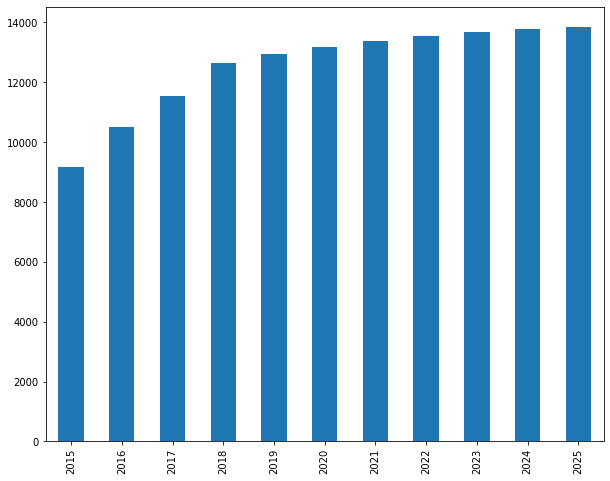
Without intervention, inactive customers grow by 51% over ten years.
Computing Revenue Projections
We need the average revenue generated by each segment:
# Calculate average 2015 revenue by segment
revenue_2015 = df[df['year_of_purchase'] == 2015].groupby('customer_id')['purchase_amount'].sum()
customers_with_revenue = customers_2015.merge(
    revenue_2015.rename('revenue_2015'),
    on='customer_id',
    how='left'
)
customers_with_revenue['revenue_2015'] = customers_with_revenue['revenue_2015'].fillna(0)

segment_revenue = customers_with_revenue.groupby('segment', observed=True)['revenue_2015'].mean()

print("\nAverage 2015 Revenue by Segment:")
print(segment_revenue.round(2))
Average 2015 Revenue by Segment:
segment
inactive                0.00
cold                    0.00
warm high value         0.00
warm low value          0.00
new warm                0.00
active high value     323.57
active low value       52.31
new active             79.17
Name: revenue_2015, dtype: float64
Active high value average $324/year. Active low value average $52. Losing 100 active high value customers costs $32,357 in annual revenue vs. only $5,231 for active low value. Now we project revenue:
# Create revenue vector (aligned with segment order in our projection matrix)
revenue_vector = segment_revenue.reindex(segment_projection.index, fill_value=0)

# Calculate revenue projection for each year
revenue_projection = segment_projection.multiply(revenue_vector, axis=0)

# Sum across segments to get total yearly revenue
yearly_revenue = revenue_projection.sum(axis=0)

print("\nProjected Yearly Revenue (2015-2025):")
print(yearly_revenue.round(0))
Projected Yearly Revenue (2015-2025):
2015    478414.00
2016    397606.00
2017    379698.00
2018    366171.00
2019    351254.00
2020    339715.00
2021    330444.00
2022    322700.00
2023    316545.00
2024    311445.00
2025    307568.00
dtype: float64
Revenue declines from $478,414 (2015) to $307,568 (2025), a 36% drop. Let’s visualize:
# Plot revenue projection
fig, ax = plt.subplots(figsize=(12, 6))
yearly_revenue.plot(kind='bar', ax=ax, color='#3498db', alpha=0.7)
ax.set_xlabel('Year', fontsize=12)
ax.set_ylabel('Revenue ($)', fontsize=12)
ax.set_title('Projected Annual Revenue (No Acquisition, No Discounting)', fontsize=14)
ax.yaxis.set_major_formatter(plt.FuncFormatter(lambda x, p: f'${x/1000:.0f}K'))
ax.grid(axis='y', alpha=0.3)
plt.tight_layout()
plt.savefig('revenue_projection.png', dpi=150, bbox_inches='tight')
plt.show()
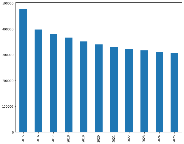
Without acquisition and retention initiatives, revenue decays by over a third.
Calculating Customer Lifetime Value with Discounting
A dollar received ten years from now is worth less than a dollar today. Discounting adjusts future cash flows to present value:
\[PV = \frac{FV}{(1 + r)^t}\]Where PV is present value, FV is future value, r is the discount rate, and t is time in years. The discount rate typically reflects your cost of capital (what you pay to borrow money) or your opportunity cost (what you could earn investing elsewhere). We’ll use 10% as a reasonable discount rate for a retail business.
# Set discount rate and calculate discount factors
discount_rate = 0.10
discount_factors = 1 / ((1 + discount_rate) ** np.arange(0, 11))

print("\nDiscount Factors (10% rate):")
discount_df = pd.DataFrame({
    'year': years,
    'discount_factor': discount_factors,
    'dollar_value': discount_factors
}).round(3)
print(tabulate(discount_df, headers='keys', tablefmt='psql', showindex=False))
Discount Factors (10% rate):
+--------+-------------------+----------------+
|   year |   discount_factor |   dollar_value |
+--------+-------------------+----------------+
|   2015 |             1.000 |          1.000 |
|   2016 |             0.909 |          0.909 |
|   2017 |             0.826 |          0.826 |
|   2018 |             0.751 |          0.751 |
|   2019 |             0.683 |          0.683 |
|   2020 |             0.621 |          0.621 |
|   2021 |             0.564 |          0.564 |
|   2022 |             0.513 |          0.513 |
|   2023 |             0.467 |          0.467 |
|   2024 |             0.424 |          0.424 |
|   2025 |             0.386 |          0.386 |
+--------+-------------------+----------------+
By 2025 (ten years out), each dollar is worth just $0.39. Now we apply discount factors to revenue:
# Calculate discounted yearly revenue
discounted_revenue = yearly_revenue * discount_factors

print("\nRevenue Comparison (Nominal vs. Present Value):")
comparison = pd.DataFrame({
    'year': years,
    'nominal_revenue': yearly_revenue,
    'discount_factor': discount_factors,
    'present_value': discounted_revenue
}).round(0)
print(tabulate(comparison, headers='keys', tablefmt='psql', showindex=False))
Revenue Comparison (Nominal vs. Present Value):
+--------+-------------------+-------------------+----------------+
|   year |   nominal_revenue |   discount_factor |   present_value |
+--------+-------------------+-------------------+-----------------|
|   2015 |        478414.00  |              1.00 |      478414.00  |
|   2016 |        397606.00  |              0.91 |      361460.00  |
|   2017 |        379698.00  |              0.83 |      313800.00  |
|   2018 |        366171.00  |              0.75 |      275110.00  |
|   2019 |        351254.00  |              0.68 |      239911.00  |
|   2020 |        339715.00  |              0.62 |      210936.00  |
|   2021 |        330444.00  |              0.56 |      186527.00  |
|   2022 |        322700.00  |              0.51 |      165596.00  |
|   2023 |        316545.00  |              0.47 |      147671.00  |
|   2024 |        311445.00  |              0.42 |      132083.00  |
|   2025 |        307568.00  |              0.39 |      118581.00  |
+--------+-------------------+-------------------+-----------------|
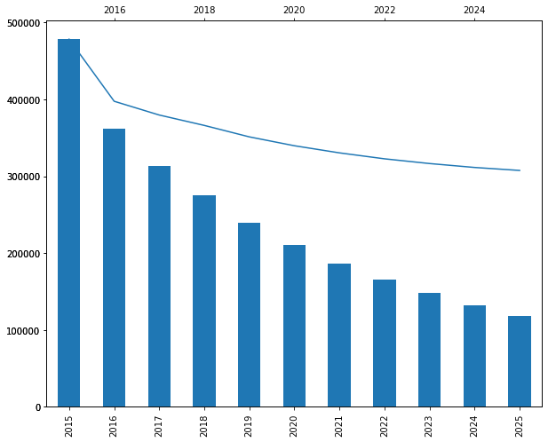
The $307,568 in 2025 nominal revenue is worth only $118,581 in present value. Let’s visualize:
# Plot nominal vs. discounted revenue
fig, ax = plt.subplots(figsize=(12, 6))

x = np.arange(len(years))
width = 0.35

bars1 = ax.bar(x - width/2, yearly_revenue, width, label='Nominal Revenue',
               color='#3498db', alpha=0.7)
bars2 = ax.bar(x + width/2, discounted_revenue, width, label='Present Value',
               color='#e74c3c', alpha=0.7)

ax.set_xlabel('Year', fontsize=12)
ax.set_ylabel('Revenue ($)', fontsize=12)
ax.set_title('Nominal vs. Discounted Revenue Projections', fontsize=14)
ax.set_xticks(x)
ax.set_xticklabels(years)
ax.yaxis.set_major_formatter(plt.FuncFormatter(lambda x, p: f'${x/1000:.0f}K'))
ax.legend()
ax.grid(axis='y', alpha=0.3)

plt.tight_layout()
plt.savefig('revenue_discounted_comparison.png', dpi=150, bbox_inches='tight')
plt.show()
Computing Total Customer Lifetime Value
CLV is the sum of all discounted future cash flows:
# Calculate cumulative metrics
cumulative_nominal = yearly_revenue.cumsum()
cumulative_pv = discounted_revenue.cumsum()

# Calculate total CLV (sum of all discounted cash flows)
total_clv = discounted_revenue.sum()
total_customers = len(customers_2015)
clv_per_customer = total_clv / total_customers

print(f"\nCustomer Lifetime Value Analysis:")
print(f"Total customer base (2015): {total_customers:,}")
print(f"Total CLV (10-year, discounted): ${total_clv:,.2f}")
print(f"Average CLV per customer: ${clv_per_customer:,.2f}")
print(f"\nComparison:")
print(f"Total nominal revenue (10-year): ${yearly_revenue.sum():,.2f}")
print(f"Discount impact: {(1 - total_clv/yearly_revenue.sum())*100:.1f}% reduction")
Customer Lifetime Value Analysis:
Total customer base (2015): 18,417
Total CLV (10-year, discounted): $2,630,089.00
Average CLV per customer: $142.80

Comparison:
Total nominal revenue (10-year): $3,661,560.00
Discount impact: 28.2% reduction
Total CLV is $2.63 million across 18,417 customers, or $142.80 per customer average. If you want a 5:1 CLV to CAC ratio, spend no more than $29 to acquire a typical customer. Let’s visualize cumulative value:
# Plot cumulative CLV over time
fig, ax = plt.subplots(figsize=(12, 6))

ax.plot(years, cumulative_pv/1000, marker='o', linewidth=2.5,
        markersize=8, color='#2ecc71', label='Cumulative CLV (Present Value)')
ax.fill_between(years, 0, cumulative_pv/1000, alpha=0.2, color='#2ecc71')

ax.set_xlabel('Year', fontsize=12)
ax.set_ylabel('Cumulative Value ($K)', fontsize=12)
ax.set_title('Cumulative Customer Lifetime Value (10-year, Discounted)', fontsize=14)
ax.grid(alpha=0.3)
ax.legend(fontsize=11)

# Add annotation for total CLV
ax.annotate(f'Total CLV: ${total_clv/1000:.0f}K',
            xy=(2025, cumulative_pv.iloc[-1]/1000),
            xytext=(2022, cumulative_pv.iloc[-1]/1000 + 200),
            fontsize=11,
            bbox=dict(boxstyle='round', facecolor='wheat', alpha=0.5),
            arrowprops=dict(arrowstyle='->', connectionstyle='arc3,rad=0.3'))

plt.tight_layout()
plt.savefig('cumulative_clv.png', dpi=150, bbox_inches='tight')
plt.show()
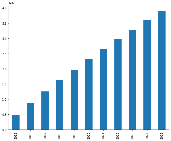
Most customer value is realized early in the relationship. The first three years generate $1.33 million (51% of total CLV). The last three years generate only $498K (19%).
Segment-Specific Lifetime Values
How much is an active high value customer worth versus an active low value customer?
# Calculate segment-specific CLV
segment_clv = revenue_projection.multiply(discount_factors, axis=1).sum(axis=1) / segment_projection[2015]
segment_clv = segment_clv.replace([np.inf, -np.inf], 0)  # Handle divide by zero

# Create comprehensive segment analysis
segment_analysis = pd.DataFrame({
    '2015_count': segment_projection[2015],
    'avg_2015_revenue': revenue_vector,
    'total_segment_clv': revenue_projection.multiply(discount_factors, axis=1).sum(axis=1),
    'clv_per_customer': segment_clv
}).round(2)

segment_analysis['pct_of_total_clv'] = (
    segment_analysis['total_segment_clv'] / segment_analysis['total_segment_clv'].sum() * 100
).round(1)

print("\nSegment-Level CLV Analysis:")
print(tabulate(segment_analysis, headers='keys', tablefmt='psql'))
Segment-Level CLV Analysis:
+-------------------+--------------+---------------------+---------------------+---------------------+---------------------+
| segment           |   2015_count |   avg_2015_revenue  |   total_segment_clv |   clv_per_customer  | pct_of_total_clv    |
+-------------------+--------------+---------------------+---------------------+---------------------+---------------------+
| inactive          |      9158.00 |                0.00 |                0.00 |                0.00 |                 0.0 |
| cold              |      1903.00 |                0.00 |                0.00 |                0.00 |                 0.0 |
| warm high value   |       119.00 |                0.00 |            43842.90 |              368.43 |                 1.7 |
| warm low value    |       901.00 |                0.00 |            40766.61 |               45.25 |                 1.5 |
| new warm          |       938.00 |                0.00 |                0.00 |                0.00 |                 0.0 |
| active high value |       573.00 |              323.57 |          1800952.04 |             3143.55 |                68.5 |
| active low value  |      3313.00 |               52.31 |           675964.03 |              204.02 |                25.7 |
| new active        |      1512.00 |               79.17 |            68563.39 |               45.34 |                 2.6 |
+-------------------+--------------+---------------------+---------------------+---------------------+---------------------+
Active high value customers average $3,144 in lifetime value. Active low value average $204. The ratio is 15:1. The 573 active high value customers (3% of the base) generate 68.5% of total value.
Implications: Losing an active high value customer forfeits $3,144. You can justify spending hundreds on personalized retention. Losing an active low value customer forfeits $204, suggesting automated retention. Acquisition targeting should focus on prospects likely to become high-value.
Business Applications
Acquisition evaluation: Strategy A acquires 1,000 discount customers at $150 each (CLV: $204). Strategy B acquires 300 premium customers at $200 each (CLV: $3,144). Strategy A net value: $54,000. Strategy B net value: $883,200. Fewer high-value customers beat many low-value customers.
Retention investment: Improving high-value retention by 10% saves 57 customers × $3,144 = $179,208. Same improvement for low-value saves 331 customers × $204 = $67,524. Focus retention on high-value first.
Product decisions: A premium product line costing $500,000 might increase high-value customer spending by 23%, generating ~$350,000 in incremental CLV (present value). Negative NPV unless it attracts additional high-value customers.
Model Limitations
Key assumptions: Stationary transition probabilities (may not hold over 10 years), no customer acquisition modeled, segment-based averaging (ignores within-segment variation), 10% discount rate (sensitivity analysis recommended).
Despite limitations, even a rough CLV estimate beats no estimate. The goal is directing resources toward high-value customers.
Conclusion
The average customer is worth $143 in present value over ten years. But active high value customers are worth $3,144 each, active low value customers $204. The 15:1 ratio means customer selection and retention have enormous financial leverage.
We used simple approaches: logistic regression, OLS, RFM segmentation, transition matrices. These workhorse methods produce interpretable results and integrate into operational systems.
Customer analytics is valuable only when it changes decisions. Start simple. Segment customers. Calculate segment-level revenue. Build transition matrices. Estimate CLV roughly. Guide a few decisions. Measure results. Iterate.
References
-
Lilien, Gary L, Arvind Rangaswamy, and Arnaud De Bruyn. 2017. Principles of Marketing Engineering and Analytics. State College, PA: DecisionPro.
-
Fader, Peter S., and Bruce G. S. Hardie. 2009. “Probability Models for Customer-Base Analysis.” Journal of Interactive Marketing 23 (1): 61-69.
-
Pfeifer, Phillip E., and Robert L. Carraway. 2000. “Modeling Customer Relationships as Markov Chains.” Journal of Interactive Marketing 14 (2): 43-55.
-
Netzer, Oded, and James M. Lattin. 2008. “A Hidden Markov Model of Customer Relationship Dynamics.” Marketing Science 27 (2): 185-204.
-
Grönroos, Christian. 1991. “The Marketing Strategy Continuum: Towards a Marketing Concept for the 1990s.” Management Decision 29 (1). https://doi.org/10.1108/00251749110139106.
-
Gupta, Sunil, Donald R. Lehmann, and Jennifer Ames Stuart. 2004. “Valuing Customers.” Journal of Marketing Research 41 (1): 7-18.
-
Arnaud De Bruyn. Foundations of Marketing Analytics (MOOC). Coursera.
-
Dataset from Github repo. Accessed 15 December 2021.
Data Science 